


SciPy 算法库和数学工具包
Scipy 是基于 Numpy 的科学计算库,用于数学、科学、工程学等领域,很多有一些高阶抽象和物理模型需要使用 Scipy。
SciPy 包含的模块有最优化、线性代数、积分、插值、特殊函数、快速傅里叶变换、信号处理和图像处理、常微分方程求解和其他科学与工程中常用的计算。
1. SciPy安装
# 下载库
python -m pip install -U scipy
# 导入库
from scipy import contants
2. 模块列表
-模块名 | -功能 |
scipy.cluster | 向量变化 |
scipy.constants | 数学常量 |
scipy.fft | 快速傅里叶变换 |
scipy.integrate | 积分 |
scipy.interpolate | 插值 |
scipy.io | 数据输入输出 |
scipy.linalg | 线性代数 |
scipy.misc | 图像处理 |
scipy.ndimage | N维图像 |
scipy.odr | 正交距离回归 |
scipy.optimize | 优化算法 |
scipy.signal | 信号处理 |
scipy.sparse | 稀疏矩阵 |
scipy.spatial | 空间数据结构和算法 |
scipy.special | 特殊数学函数 |
scipy.stats | 统计函数 |
3. SciPy常量模块
SciPy常量模块contants提供了许多内置数学常数。还包括国际单位制词头和二进制前缀字节单位。
圆周率
print(constants.pi) # 3.141592653589793黄金比例
print(constants.golden) # 1.618033988749895使用dir()函数可以查看contants模块包含了那些常量、
print(dir(constants))质量单位
print(constants.gram)        #0.001    kg
print(constants.metric_ton)  #1000.0   公吨
角度单位
print(constants.degree)     #0.017453292519943295  弧度
print(constants.arcmin)     #0.0002908882086657216  弧分
时间单位
print(constants.minute)      #60.0
print(constants.hour)        #3600.0
print(constants.day)         #86400.0
print(constants.week)        #604800.0
print(constants.year)        #31536000.0
print(constants.Julian_year) #31557600.0   儒略年
长度单位
print(constants.inch)              #0.0254  英寸
print(constants.foot)              #0.30479  英尺
压强单位
print(constants.atm)         #101325.0  帕斯卡
print(constants.atmosphere)  #101325.0
面积单位
print(constants.hectare) #10000.0  公顷
print(constants.acre)    #4046.8564223999992  英亩
体积单位
print(constants.kmh)            #0.2778
print(constants.mph)            #0.447
温度、能量单位(两者公式一样,温度是开尔文,能量是焦耳)
print(constants.zero_Celsius)      #273.15  零度
print(constants.degree_Fahrenheit) #0.5555  华氏度
力学单位
print(constants.dyn)             #1e-05  达因
print(constants.dyne)            #1e-05  达因
4. SciPy优化器
NumPy 能够找到多项式和线性方程的根,但它无法找到非线性方程的根。
因此我们可以使用 SciPy 的 optimze.root 函数,这个函数需要两个参数:
fun - 表示方程的函数。
x0 - 根的初始猜测。
该函数返回一个对象,其中包含有关解决方案的信息。
x + cos(x)  # numpy无法得出根


from scipy.optimize import root
from math import cos

def eqn(x):
  return x + cos(x)

myroot = root(eqn, 0)
print(myroot.x)     # -0.73908513]
# 查看更多信息
#print(myroot)
最小化函数
函数表示一条曲线,曲线有高点和低点。
整条曲线中的最高点称为全局最大值,其余部分称为局部最大值。整条曲线的最低点称为全局最小值,其余的称为局部最小值。
minimize() 函数接受以下几个参数:
fun - 要优化的函数
x0 - 初始猜测值
method - 要使用的方法名称,值可以是:'CG','BFGS','Newton-CG','L-BFGS-B','TNC','COBYLA',,'SLSQP'。
callback - 每次优化迭代后调用的函数。
options - 定义其他参数的字典:
{ "disp": boolean - print detailed description "gtol": number - the tolerance of the error }
实例
# x^2 + x + 2 使用 BFGS 的最小化函数:

from scipy.optimize import minimize

def eqn(x):
  return x**2 + x + 2

mymin = minimize(eqn, 0, method='BFGS')
print(mymin)

# 输出结果
	  fun: 1.75
 hess_inv: array([[0.50000001]])
      jac: array([0.])
  message: 'Optimization terminated successfully.'
     nfev: 8
      nit: 2
     njev: 4
   status: 0
  success: True
        x: array([-0.50000001])
五. SciPy稀疏矩阵
指在数值分析中绝大多数数值为零的矩阵。反之,如果大部分元素都非零,则这个矩阵是稠密的(Dense)
SciPy 的 scipy.sparse 模块提供了处理稀疏矩阵的函数。
我们主要使用以下两种类型的稀疏矩阵:
CSC - 压缩稀疏列(Compressed Sparse Column),按列压缩。
CSR - 压缩稀疏行(Compressed Sparse Row),按行压缩。
CSR矩阵
通过向 scipy.sparse.csr_matrix() 函数传递数组来创建一个 CSR 矩阵。
import numpy as np
from scipy.sparse import csr_matrix

arr = np.array([0, 0, 0, 0, 0, 1, 1, 0, 2])

print(csr_matrix(arr))

# 结果
  (0, 5)        1
  (0, 6)        1
  (0, 8)        2
第一行:在矩阵第一行(索引值 0 )第六(索引值 5 )个位置有一个数值 1。
第二行:在矩阵第一行(索引值 0 )第七(索引值 6 )个位置有一个数值 1。
第三行:在矩阵第一行(索引值 0 )第九(索引值 8 )个位置有一个数值 2。
CSR矩阵分析方法
使用data属性查看存储数据(不含0元素)
arr = np.array([[0, 0, 0], [0, 0, 1], [1, 0, 2]])

print(csr_matrix(arr).data)

# 输出结果
[1 1 2]
使用 count_nonzero() 方法计算非 0 元素的总数:
arr = np.array([[0, 0, 0], [0, 0, 1], [1, 0, 2]])

print(csr_matrix(arr).count_nonzero())

# 结果
3
使用 eliminate_zeros() 方法删除矩阵中 0 元素:
arr = np.array([[0, 0, 0], [0, 0, 1], [1, 0, 2]])

mat = csr_matrix(arr)
mat.eliminate_zeros()

print(mat)

# 输出结果
  (1, 2)    1
  (2, 0)    1
  (2, 2)    2
使用 sum_duplicates() 方法来删除重复项
arr = np.array([[0, 0, 0], [0, 0, 1], [1, 0, 2]])

mat = csr_matrix(arr)
mat.sum_duplicates()

print(mat)

# 输出结果
  (1, 2)    1
  (2, 0)    1
  (2, 2)    2
csr 转换为 csc 使用 tocsc() 方法:
arr = np.array([[0, 0, 0], [0, 0, 1], [1, 0, 2]])

newarr = csr_matrix(arr).tocsc()

print(newarr)

# 输出结果
  (2, 0)    1
  (1, 2)    1
  (2, 2)    2
6. SciPy 图结构
SciPy 提供了 scipy.sparse.csgraph 模块来处理图结构。
邻接矩阵
邻接矩阵(Adjacency Matrix)是表示顶点之间相邻关系的矩阵。
邻接矩阵又分为有向图邻接矩阵和无向图邻接矩阵。
Dijkstra -- 最短路径算法
Dijkstra(迪杰斯特拉)最短路径算法,用于计算一个节点到其他所有节点的最短路径。
Scipy 使用 dijkstra() 方法来计算一个元素到其他元素的最短路径。
dijkstra() 方法可以设置以下几个参数:
return_predecessors: 布尔值,设置 True,遍历所有路径,如果不想遍历所有路径可以设置为 False。
indices: 元素的索引,返回该元素的所有路径。
limit: 路径的最大权重。
import numpy as np
from scipy.sparse.csgraph import dijkstra
from scipy.sparse import csr_matrix

arr = np.array([
  [0, 1, 2],
  [1, 0, 0],
  [2, 0, 0]
])

newarr = csr_matrix(arr)

print(dijkstra(newarr, return_predecessors=True, indices=0))

# 输出结果
# (array([ 0.,  1.,  2.]), array([-9999,     0,     0], dtype=int32))
Floyd Warshall -- 佛洛依德算法
弗洛伊德算法是解决任意两点间的最短路径的一种算法。
Scipy 使用 floyd_warshall() 方法来查找所有元素对之间的最短路径。
# 查找所有元素对之间的最短路径
from scipy.sparse.csgraph import floyd_warshall

arr = np.array([
  [0, 1, 2],
  [1, 0, 0],
  [2, 0, 0]
])

newarr = csr_matrix(arr)

print(floyd_warshall(newarr, return_predecessors=True))

# 输出结果
# (array([[ 0.,  1.,  2.],
#       [ 1.,  0.,  3.],
#       [ 2.,  3.,  0.]]), array([[-9999,     0,     0],
#       [    1, -9999,     0],
#       [    2,     0, -9999]], dtype=int32))
Bellman Ford -- 贝尔曼-福特算法
贝尔曼-福特算法是解决任意两点间的最短路径的一种算法。
Scipy 使用 bellman_ford() 方法来查找所有元素对之间的最短路径。
from scipy.sparse.csgraph import bellman_ford
arr = np.array([
  [0, -1, 2],
  [1, 0, 0],
  [2, 0, 0]
])

newarr = csr_matrix(arr)

print(bellman_ford(newarr, return_predecessors=True, indices=0))

# 输出结果
# (array([ 0., -1.,  2.]), array([-9999,     0,     0], dtype=int32))
深度优先顺序
depth_first_order() 方法从一个节点返回深度优先遍历的顺序。
from scipy.sparse.csgraph import depth_first_order
arr = np.array([
  [0, 1, 0, 1],
  [1, 1, 1, 1],
  [2, 1, 1, 0],
  [0, 1, 0, 1]
])

newarr = csr_matrix(arr)

print(depth_first_order(newarr, 1))

# 输出结果
(array([1, 0, 3, 2], dtype=int32), array([    1, -9999,     1,     0], dtype=int32))
广度优先顺序
breadth_first_order() 方法从一个节点返回广度优先遍历的顺序
from scipy.sparse.csgraph import breadth_first_order
arr = np.array([
  [0, 1, 0, 1],
  [1, 1, 1, 1],
  [2, 1, 1, 0],
  [0, 1, 0, 1]
])

newarr = csr_matrix(arr)

print(breadth_first_order(newarr, 1))

# 输出结果
# (array([1, 0, 2, 3], dtype=int32), array([    1, -9999,     1,     1], dtype=int32))
6. SciPy空间数据
空间数据又称几何数据,它是用来表示物体的位置、形态、大小分布等各方面信息,比如坐标上的点。SciPy 通过 scipy.spatial 模块处理空间数据。
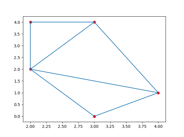
三角测量
# 通过给定的点来创建三角函数
import numpy as np
from scipy.spatial import Delaunay
import matplotlib.pyplot as plt

points = np.array([
  [2, 4],
  [3, 4],
  [3, 0],
  [2, 2],
  [4, 1]
])

simplices = Delaunay(points).simplices    # 三角形中顶点的索引

plt.triplot(points[:, 0], points[:, 1], simplices)
plt.scatter(points[:, 0], points[:, 1], color='r')

plt.show()
输出结果
凸包
from scipy.spatial import ConvexHull
points = np.array([
  [2, 4],
  [3, 4],
  [3, 0],
  [2, 2],
  [4, 1],
  [1, 2],
  [5, 0],
  [3, 1],
  [1, 2],
  [0, 2]
])

hull = ConvexHull(points)
hull_points = hull.simplices

plt.scatter(points[:,0], points[:,1])
for simplex in hull_points:
  plt.plot(points[simplex,0], points[simplex,1], 'k-')

plt.show()
输出结果

K-D树
from scipy.spatial import KDTree
points = [(1, -1), (2, 3), (-2, 3), (2, -3)]
kdtree = KDTree(points)
res = kdtree.query((1, 1))
print(res)
# 输出结果
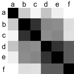
(2.0, 0)距离矩阵
一个距离矩阵是一个各项元素为点之间距离的矩阵(二维数组)。
距离矩阵的这些数据可以进一步被看成是图形表示的热度图(如下图所示),其中黑色代表距离为零,白色代表最大距离。
欧几里得距离
即欧几里得空间中两点的直线距离。
欧几里得度量(也称欧式距离):指在m维空间中两个点之间的真实距离,或者向量的自然长度。
from scipy.spatial.distance import euclidean
p1 = (1, 0)
p2 = (10, 2)
res = euclidean(p1, p2)
print(res)
# 输出结果
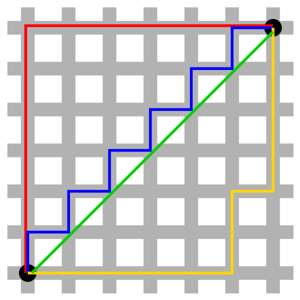
# 9.21954445729曼哈顿距离
用以标明两个点在标准坐标系上的绝对轴距总和。曼哈顿距离 只能上、下、左、右四个方向进行移动,并且两点之间的曼哈顿距离是两点之间的最短距离。
曼哈顿与欧几里得距离: 红、蓝与黄线分别表示所有曼哈顿距离都拥有一样长度(12),而绿线表示欧几里得距离有6×√2 ≈ 8.48的长度。
# 实例计算曼哈顿距离
from scipy.spatial.distance import cityblock

p1 = (1, 0)
p2 = (10, 2)
res = cityblock(p1, p2)
print(res)

# 输出结果
11
余弦距离
余弦距离,也称为余弦相似度,通过测量两个向量的夹角的余弦值来度量它们之间的相似性。
0 度角的余弦值是 1,而其他任何角度的余弦值都不大于 1,并且其最小值是 -1。
from scipy.spatial.distance import cosine

p1 = (1, 0)
p2 = (10, 2)
res = cosine(p1, p2)
print(res)
# 输出结果
# 0.019419324309079777
汉明距离
在信息论中,两个等长字符串之间的汉明距离是两个字符串对应位置的不同字符的个数。换句话说,他是将一个字符串编程另一个字符串所需要替换的字符串个数。
汉明重量是字符串组对于同样长度的零字符串的汉明距离,即字符串中非零元素的个数。对于二进制就是1的个数。
from scipy.spatial.distance import hamming

p1 = (True, False, True)
p2 = (False, True, True)
res = hamming(p1, p2)
print(res)

# 0.666666666667
7. SciPy Matlab 数组
NumPy 提供了 Python 可读格式的数据保存方法。
SciPy 提供了与 Matlab 的交互的方法。
SciPy 的 scipy.io 模块提供了很多函数来处理 Matlab 的数组
以Matlab格式导出数据
savemat() 方法可以导出 Matlab 格式的数据。
该方法参数有:
filename - 保存数据的文件名。
mdict - 包含数据的字典。
do_compression - 布尔值,指定结果数据是否压缩。默认为 False。
# 将数组作为变量‘vec’导出到mat文件

from scipy import io
import numpy as np

arr = np.arange(10)

io.savemat('arr.mat', {"vec": arr})
导入Matlab格式数据
loadmat() 方法可以导入 Matlab 格式数据。
该方法参数:
filename - 保存数据的文件名。返回一个数组。
# 实例从mat文件中导入数组

arr = np.array([0, 1, 2, 3, 4, 5, 6, 7, 8, 9,])
# 导出
io.savemat('arr.mat', {"vec": arr})
# 导入
mydata = io.loadmat('arr.mat')
print(mydata)

# 使用变量名vec只显示matlab数据的数组
print(mydata['vec'])  # [[0 1 2 3 4 5 6 7 8 9]]
8. SciPy插值
插值(interpolation)是一种已知的、离散的数据点。简单来说插值就是一种在给定的点之间生成点的方法。
SciPy 提供了 scipy.interpolate 模块来处理插值。
一维插值
一位数据的插值运算可以通过方法interpld()完成。该方法接收两个参数x和y,返回值是可调用函数,该函数可以用新的x调用并返回相应的y,y=f(x)。
from scipy.interpolate import interp1d
import numpy as np

xs = np.arange(10)
ys = 2*xs + 1
interp_func = interp1d(xs, ys)
newarr = interp_func(np.arange(2.1, 3, 0.1))
print(newarr)

# 输出结果
[5.2  5.4  5.6  5.8  6.   6.2  6.4  6.6  6.8]
# 注意:新的 xs 应该与旧的 xs 处于相同的范围内,这意味着我们不能使用大于 10 或小于 0 的值调用 interp_func()。
单变量插值
单变量插值使用 UnivariateSpline() 函数
from scipy.interpolate import UnivariateSpline
import numpy as np

xs = np.arange(10)
ys = xs**2 + np.sin(xs) + 1

interp_func = UnivariateSpline(xs, ys)

newarr = interp_func(np.arange(2.1, 3, 0.1))

print(newarr)

# 输出结果
[5.62826474 6.03987348 6.47131994 6.92265019 7.3939103  7.88514634
   8.39640439 8.92773053 9.47917082]
径向基函数插值
是一种非线性插值技术,它将像素点的值基于它们之间的相对位置,而不是照片空间中的绝对位置。
from scipy.interpolate import Rbf
import numpy as np

xs = np.arange(10)
ys = xs**2 + np.sin(xs) + 1

interp_func = Rbf(xs, ys)

newarr = interp_func(np.arange(2.1, 3, 0.1))

print(newarr)

# 输出结果
  [6.25748981  6.62190817  7.00310702  7.40121814  7.8161443   8.24773402
   8.69590519  9.16070828  9.64233874]
9.Scipy显著性检验
显著性检验就是事先对总体(随机变量)的参数或总体分布形式做出一个假设,然后利用样本信息来判断这个假设是否合理,即判断总体的真实情况与原假设是否有显著性差异。显著性检验是针对我们对总体所做的假设做检验,器原理就是“小概率时间实际不可能性原理”来接收或否定假设。
SciPy 提供了 scipy.stats 的模块来执行Scipy 显著性检验的功能。
统计假设
统计假设是关于一个或多个随机变量的位置分布的假设。随机变量的分布形式一直,而仅涉及分布中的一个或几个位置参数的统计假设,称为参数假设。
零假设
零假设,又称原假设,指进行统计检验室预先建立的假设。零假设成立时,有关统计量因服从一直的某种概率分布。当统计的计算值落入否定域时,即发生了小概率时间,应否定原假设。
通常吧一个要检验的假设记作H0,称为原假设(或零假设),与H0对立的假设记作H1,称为被择假设。
在原假设为真时,决定放弃原假设,称为第一类错误,其出现的概率通常记作 α;
在原假设不真时,决定不放弃原假设,称为第二类错误,其出现的概率通常记作 β
α+β 不一定等于 1。
备择假设
备择假设包含关于总体分布的一切使原假设不成立的命题。备择假设亦称为对立假设、备选假设。备选假设可以替代零假设。
单边假设
单边检验亦称为单尾检验,用检验统计量的密度曲线和二轴所围成面积中的单侧尾部面积来构造临界区域进行检验的方法称为单边检验。
当我们的假设仅测试值的一侧时,它被称为"单尾测试"
双边检验
双边检验(two-sided test),亦称双尾检验、双侧检验在假设检验中,用检验统计量的密度曲线和x轴所围成的面积的左右两边的尾部面积来构造临界区域进行检验的方法。
阿尔法值
阿尔法值是显著性水平。
显著性水平是估计总体参数落在某一区间内,可能犯错的概率,用α表示。数据必须有多接近极端才能拒绝零假设。通常取值为0.01、0.05或0.1
P值
P值表明数据实际接近极端的程度。
比较P值和阿尔法值来确定统计显著性水平。
如果 p 值 <= alpha,我们拒绝原假设并说数据具有统计显著性,否则我们接受原假设。
T检验(T-Test)
T检验用于确定两个变量的均值之间是否存在显著性差异,并判断它们是否属于同一分布。它是双尾测试。
函数 ttest_ind() 获取两个相同大小的样本,并生成 t 统计和 p 值的元组。
# 查找给定值v1和v2是否来自相同的分布
import numpy as np
from scipy.stats import ttest_ind

v1 = np.random.normal(size=100)
v2 = np.random.normal(size=100)
res = ttest_ind(v1, v2)
print(res)

# 输出结果
Ttest_indResult(statistic=0.40833510339674095, pvalue=0.68346891833752133)
# 如果只想显示P值
v1 = np.random.normal(size=100)
v2 = np.random.normal(size=100)
res = ttest_ind(v1, v2).pvalue
print(res) # 0.68346891833752133KS检验
KS检验用于检查给定值是否符合分布。该函数接受两个参数;测试的值和CDF。CDF为累积分布函数,又叫分布函数。CDF可以是字符串,也可以是返回概率的可调用函数。也可以用作单尾或者双尾测试(默认双尾测试)。
# 查找给定值是否符合正态分布
import numpy as np
from scipy.stats import kstest

v = np.random.normal(size=100)
res = kstest(v, 'norm')
print(res)

# 输出结果
KstestResult(statistic=0.047798701221956841, pvalue=0.97630967161777515)
数据统计说明
使用describe()函数可以查看数组的信息。
import numpy as np
from scipy.stats import describe

v = np.random.normal(size=100)
res = describe(v)

print(res)

# 输出结果
DescribeResult(
    nobs=100,
    minmax=(-2.0991855456740121, 2.1304142707414964),
    mean=0.11503747689121079,
    variance=0.99418092655064605,
    skewness=0.013953400984243667,
    kurtosis=-0.671060517912661
  )
正态性检验(偏度和峰度)
利用观测数据判断总体是否服从正态分布的检验称为正态性检验,它是统计判决中重要的一种特殊的拟合优度假设检验。正态性检验基于偏度和峰度。normaltest() 函数返回零假设的 p 值。
偏度
数据对称性的度量,正态分布则是0,为负左偏,为正则意味着数据正确倾斜。
峰度
衡量数据是重尾韩式轻尾正态分布的度量。正峰度即重尾,负峰度意味着轻尾。
# 查找数组中值的偏度和峰度
import numpy as np
from scipy.stats import skew, kurtosis

v = np.random.normal(size=100)
print(skew(v)) # 0.11168446328610283
print(kurtosis(v)) #  -0.1879320563260931


# 查找数据是否来自正态分布
from scipy.stats import normaltest

v = np.random.normal(size=100)
print(normaltest(v)

# 输出结果
# NormaltestResult(statistic=4.4783745697002848, pvalue=0.10654505998635538)


 4246
4246


 被折叠的 条评论
为什么被折叠?
被折叠的 条评论
为什么被折叠?
 到【灌水乐园】发言


