


文章目录
简介
本节是新加的内容,根据老师的描述Anomaly Detection就是要机器知道它不知道这件事情。

公式输入请参考:在线Latex公式
Problem Formulation
Given a set of training data:
{
x
1
,
x
2
,
⋯
,
x
N
}
\{x^1,x^2,\cdots,x^N\}
{x1,x2,⋯,xN}
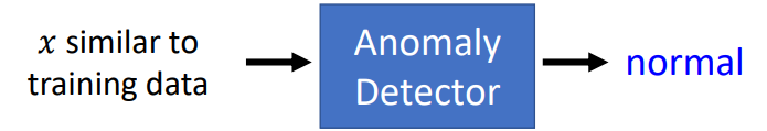
• We want to find a function detecting input 𝑥 is similar to training data or not.
这个事情如果从机器学习的角度来看,实际上是要机器去找一个function(蓝色框框)
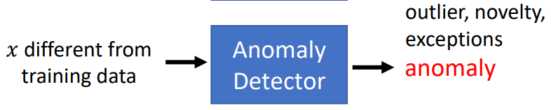
Different approaches use different ways to determine the similarity.
Anomaly Detection不一定是找不好的东西,例如novelty是找出新颖的对象。
下面来看什么叫做异常?取决于数据,例如:

应用
• Fraud Detection
Training data: 正常刷卡行為, 𝑥: 盜刷?
Ref: https://www.kaggle.com/ntnu-testimon/paysim1/home
Ref: https://www.kaggle.com/mlg-ulb/creditcardfraud/home
• Network Intrusion Detection
Training data: 正常連線, 𝑥: 攻擊行為?
Ref: http://kdd.ics.uci.edu/databases/kddcup99/kddcup99.html
• Cancer Detection
Training data: 正常細胞, 𝑥: 癌細胞
Ref: https://www.kaggle.com/uciml/breast-cancer-wisconsin-data/home
如何做Anomaly Detection
思路1看做二分类的方法来弄。
二分类
Given normal data
{
x
1
,
x
2
,
⋯
,
x
N
}
\{x^1,x^2,\cdots,x^N\}
{x1,x2,⋯,xN}
Given anomaly
{
x
~
1
,
x
~
2
,
⋯
,
x
~
N
}
\{\tilde x^1,\tilde x^2,\cdots,\tilde x^N\}
{x~1,x~2,⋯,x~N}
Then training a binary classifier ……就这样结束?
不可以这样玩,例如:
正常的数据
x
x
x是宝可梦:

那么异常的数据
x
~
\tilde x
x~是除了宝可梦之外的一切事物:

神奇宝贝、凉宫春日、茶壶。。。。这些东西cannot be considered as a class.
原因:
1、无法穷举非宝可梦的对象,无法把异常视为一个类别。
2、很难收集到anomaly 的数据。Even worse, in some cases, it is difficult to find anomaly example ……
看来二分类不行,那么Anomaly Detection有几种?
Categories
第一种:称为:Open-set Recognition,每一个训练数据都有对应的标签,那么我们可以训练一个Classifier(可以用NN,也可以用线性分类器),这个Classifier训练好后,如果看到训练数据中不存在的数据,那么可以为其打上【unknown】的标签。
第二种:只有训练数据,没有标签。这里又分两种情况:
- All the training data is normal.所有数据都是正常数据。
- A little bit of training data is anomaly. 有一些数据是异常数据。

下面分别对各个类别进行讲解。
Case 1: With Classifier
Example Application
判断卡通人物是否来自辛普森家庭


现在有数据及标签:

然后要训练分类器:

Source of model: https://www.kaggle.com/alexattia/the-simpsons-characters-dataset/
有人做了这个分类器,准确率还不错:96%:

修改这个分类器,使其在输入人物是属于辛普森家庭中的哪一个,还要输出对分类结果的信心分数
c
c
c。

然后根据信心分数来进行异常检测:
f
(
x
)
=
{
n
o
r
m
a
l
c
(
x
)
>
λ
a
n
o
m
a
l
y
c
(
x
)
≤
λ
f(x)=\begin{cases} normal & c(x)>\lambda \\ anomaly & c(x)\leq\lambda \end{cases}
f(x)={normalanomalyc(x)>λc(x)≤λ
估计信心分数
由于Classifier的输出实际上是一个分布(softmax),所以会有:

如果丢一张怪怪的图片:

也就是说softmax输出的最大值就是信心分数(上图中的红框)。
或者算分类几率的熵,熵越大说明越混乱,越无法确定分类。
其实用哪种方法没有很大差别,这里用第一种,方便:


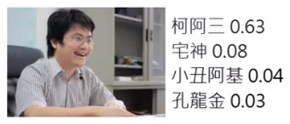
由以上结果看到如果输入是辛普森家族中的人物,信心分数会比较高,反之比较低。
但是也有例外:

老师说,但凡是出现机器识别错误的情况,一般都会把非辛普森家族人物识别为柯阿三

因为它是辛普森家族中唯一一个不是黄脸的人物,所以一旦出现非辛普森家族人物,机器认错的话就会认为是柯阿三。
上面的凉宫春日的头发是棕色,和柯阿三的脸颜色差不多,所以会出错。
在网上发布的辛普森数据集中,把所有数据丢到当前Classifier中得到的信心分数结果如下图:
Confidence score distribution for characters from Simpsons :

可以看到结果是非常集中的,当然也有错误的地方(红色)
Confidence score distribution for anime characters:

上面的丢随意的动漫人物进去得到的结果,丢了1万5千张,只有1400张左右是识别为辛普森家族人物。多数输入的信心分数比较低。
上面用分类器求信心分数的方法简单实用,是实作的首选,当然还有更复杂的方法:
Outlook: Network for Confidence Estimation
文献:Terrance DeVries, Graham W. Taylor, Learning Confidence for Out-of-Distribution Detection in Neural Networks, arXiv, 2018
• Learning a network that can directly output confidence
在训练NN的时候就直接训练NN输出信心分数。(不展开)

Example Framework
小结一下辛普森家庭人物异常检测模型的框架:
Training Set: Images
x
x
x of characters from Simpsons.Each image
x
x
x is labelled by its characters
y
^
\hat y
y^.
Train a classifier, and we can obtain confidence score
c
(
x
)
c(x)
c(x)from the classifier.
f
(
x
)
=
{
n
o
r
m
a
l
c
(
x
)
>
λ
a
n
o
m
a
l
y
c
(
x
)
≤
λ
f(x)=\begin{cases} normal & c(x)>\lambda \\ anomaly & c(x)\leq\lambda \end{cases}
f(x)={normalanomalyc(x)>λc(x)≤λ
Dev Set: Images
x
x
x
Label each image
x
x
x is from Simpsons or not. (图片x是要带标签的:是否来自辛普森家族)
We can compute the performance of
f
(
x
)
f(x)
f(x).
Using dev set to determine
λ
\lambda
λ and other hyperparameters.
训练的时候数据是都来自辛普森家族,调参的时候都要有。
Testing Set: Image
x
→
x \rightarrow
x→ from Simpsons or not. #
Evaluation
上面的Dev Set部分要根据performance of
f
(
x
)
f(x)
f(x)来调整
λ
\lambda
λ ,下面来看怎么做:
100 Simpsons,5 anomalies(红色).

虽然最右边那个美女的信心分数是0.998,但是模型对于大多数的辛普森家族人物识别的信心分数是大于0.998的。
所以不是说有人物识别出来的信心分数很高就说这个分类器很烂,而是我们可以设置
λ
\lambda
λ的阈值大于0.998,来确保其他人物的分类是非辛普森家族人物。

Cost的判断
Accuracy is not a good measurement!
A system can have high accuracy, but do nothing.
因为异常值比较少。例如上图中的,如果5个异常值全部识别错误:
5 wrong, 100 correct. Accuracy:
100
100
+
5
=
95.2
%
\cfrac{100}{100+5}=95.2\%
100+5100=95.2%
因此我们要分开来看,如果现在
λ
\lambda
λ在如下图所示的位置:

那么我们可以根据异常值和正常值,是否被发现来做表格:
| Anomaly | Normal | |
|---|---|---|
| Detected | 1 | 1 (False alarm)正常判断为错误 |
| not | 4 (Missing)错误未判断 | 99 |
把
λ
\lambda
λ换个地方

| Anomaly | Normal | |
|---|---|---|
| Detected | 2 | 6 (False alarm)正常判断为错误 |
| not | 3 (Missing)错误未判断 | 94 |
这两个系统哪个好要取决我们对False alarm或是Missing的容忍度。
我们可以把容忍度做Cost表格A:
| Cost | Anomaly | Normal |
|---|---|---|
| Detected | 0 | 100 |
| not | 1 | 0 |
意思是异常值Missing记1分,正常值False alarm记100分,那么系统1的cost为104,而系统2的cost为603。系统1比较好
如果用另外一个Cost表格B:
| Cost | Anomaly | Normal |
|---|---|---|
| Detected | 0 | 1 |
| not | 100 | 0 |
意思是异常值Missing记100分,正常值False alarm记1分,那么系统1的cost为401,而系统2的cost为306。系统2比较好。
Cost表格B比较适合惩罚Missing的情况,例如癌症未检测比无并检测为癌症要严重。
Some evaluation metrics consider the ranking. For example, Area under ROC curve
其他问题
理想的分类器是这样子的,下面是猫狗分类器:

如果有些动物没有猫的特征也没有狗的特征:

那我们会把这些东西放在边界上,分数会比较低。
但是有些动物有虽然不是猫狗但是有猫狗的特征,例如老虎和狼。而且老虎比猫还要像猫,狼比狗还要像狗。
所以老虎和狼在分类器上的信心分数比猫和狗还高。

回到辛普森分类的例子,如果把二次元人物和老师的头像改变一下,结果是:

意思就是如果分类器是按黄色来进行区分是否辛普森家族人物的时候,如果有些图片不是辛普森人物,但是也明显带有黄色的特征,就会分类出错,如何解决这个问题?(不展开)
就是教机器两个事情(文献:Kimin Lee, Honglak Lee, Kibok Lee, Jinwoo Shin, Training Confidencecalibrated Classifiers for Detecting Out-of-Distribution Samples, ICLR 2018):
1、正确的对象信心分数要越高越好;(这个之前就说了)
2、异常的对象信心分数要越低越好。Learn a classifier giving low confidence score to anomaly.
但是之前说了,异常对象不好收集。有人提出用训练一个生成模型生成一些异常对象。(文献:Mark Kliger, Shachar Fleishman, Novelty Detection with GAN, arXiv, 2018)
Case 2: Without Labels
Twitch Plays Pokémon

一款网络游戏,主角是由N个人同时操控,系统会选择其中一个指令进行操作。
·Why is the game so difficult?
答:Probably because of “Troll”(网络小白)
· Players that are not familiar with the game
· Just for fun .…
· Malicious players…
in all, the players who don’t want to complete the game.
假设想要通关的玩家的操作是正常数据,能否使用异常检测找到Troll?
下面看如何解决这个问题
Problem Formulation
Given a set of training data:
{
x
1
,
x
2
,
⋯
,
x
N
}
\{x^1,x^2,\cdots,x^N\}
{x1,x2,⋯,xN}.
We want to find a function detecting input
x
x
x is similar to training data or not.
这里的输入信息
x
x
x 是一个玩家

也就是每一个玩家要先表示成一个feature vector,才能进行机器学习

例如第一维
x
1
x_1
x1可以表示为说垃圾话的频率;
第二维
x
2
x_2
x2可以表示为无政府状态下的发言频率。(这里系统操作角色有两种模式,一种是取所有输入操作中取操作最多的动作进行操作,例如:100个玩家有90个输入←,那么游戏角色就向←走,一种是随机模式(无政府状态),不管输入操作的多少,都随机选一个进行操作。有研究表明,在无政府状态下,troll倾向于发起操作。)
现在我们有大量的输入,但是没有标签y,我们可以建立一个几率模型
P
(
x
)
P(x)
P(x),用来表示某一个玩家操作发生的几率,然后根据
P
(
x
)
P(x)
P(x)来设置阈值看玩家是否是异常。

然后把所有玩家的
x
1
x_1
x1和
x
2
x_2
x2的分布可视化出来:

从图中可以看到,
P
(
x
)
P(x)
P(x)大的玩家可能是正常玩家(左上角的点),反之是异常玩家。
下面要像更加精确的用数字来表达这个事情,就要用的MLE:
Assuming the data points is sampled from a probability density function
f
θ
(
x
)
f_\theta(x)
fθ(x)
•
θ
\theta
θ determines the shape of
f
θ
(
x
)
f_\theta(x)
fθ(x)
•
θ
\theta
θ is unknown, to be found from data

L
(
θ
)
=
f
θ
(
x
1
)
f
θ
(
x
2
)
⋯
f
θ
(
x
N
)
(1)
L(\theta)=f_\theta(x^1)f_\theta(x^2)\cdots f_\theta(x^N)\tag1
L(θ)=fθ(x1)fθ(x2)⋯fθ(xN)(1)
要找
θ
∗
\theta^*
θ∗使得PDF最大:
θ
∗
=
a
r
g
max
θ
L
(
θ
)
(2)
\theta^*=arg\underset{\theta}{\text{max}}L(\theta)\tag2
θ∗=argθmaxL(θ)(2)
我们假设分布是高斯分布
f
μ
,
Σ
(
x
)
=
1
(
2
π
)
D
/
2
1
∣
Σ
∣
1
/
2
e
x
p
{
−
1
2
(
x
−
μ
)
T
Σ
−
1
(
x
−
μ
)
}
D
is the dimension of
x
f_{\mu,\Sigma}(x)=\cfrac{1}{(2\pi)^{D/2}}\cfrac{1}{|\Sigma|^{1/2}}exp\left \{-\cfrac{1}{2}(x-\mu)^T\Sigma^{-1}(x-\mu) \right \}\\ D\text{ is the dimension of }x
fμ,Σ(x)=(2π)D/21∣Σ∣1/21exp{−21(x−μ)TΣ−1(x−μ)}D is the dimension of x
这个分布看上去很复杂,但是我们只需要把它看做是输入为向量x,输出是这个向量x被sample到的几率。Input: vector x, output: probability density of sampling x.
θ
\theta
θ which determines the shape of the function are mean
μ
\mu
μ and covariance matrix
Σ
\Sigma
Σ
公式(1)就可以写成:
L
(
μ
,
Σ
)
=
f
μ
,
Σ
(
x
1
)
f
μ
,
Σ
(
x
2
)
⋯
f
μ
,
Σ
(
x
N
)
L(\mu,\Sigma)=f_{\mu,\Sigma}(x^1)f_{\mu,\Sigma}(x^2)\cdots f_{\mu,\Sigma}(x^N)
L(μ,Σ)=fμ,Σ(x1)fμ,Σ(x2)⋯fμ,Σ(xN)
公式(2)可以写成:
μ
∗
,
Σ
∗
=
a
r
g
max
μ
,
Σ
L
(
μ
,
Σ
)
\mu^*,\Sigma^*=arg\underset{\mu,\Sigma}{\text{max}}L(\mu,\Sigma)
μ∗,Σ∗=argμ,ΣmaxL(μ,Σ)

注:当然,也可以假设参数
θ
\theta
θ不是高斯分布产生的,可以是更加复杂的网络参生的(不展开)。
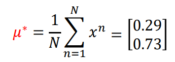
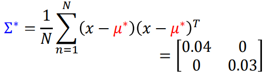
μ
∗
,
Σ
∗
\mu^*,\Sigma^*
μ∗,Σ∗可以直接根据MLE的公式算出来,直接贴结果:
最后就可以把x代入下面的判断条件,来决定是否是异常玩家。
f
μ
∗
,
Σ
∗
(
x
)
=
1
(
2
π
)
D
/
2
1
∣
Σ
∗
∣
1
/
2
e
x
p
{
−
1
2
(
x
−
μ
∗
)
T
Σ
−
1
(
x
−
μ
∗
)
}
f_{\mu^*,\Sigma^*}(x)=\cfrac{1}{(2\pi)^{D/2}}\cfrac{1}{|\Sigma^*|^{1/2}}exp\left \{-\cfrac{1}{2}(x-\mu^*)^T\Sigma^{-1}(x-\mu^*) \right \}
fμ∗,Σ∗(x)=(2π)D/21∣Σ∗∣1/21exp{−21(x−μ∗)TΣ−1(x−μ∗)}
f
(
x
)
=
{
n
o
r
m
a
l
f
μ
∗
,
Σ
∗
(
x
)
>
λ
a
n
o
m
a
l
y
f
μ
∗
,
Σ
∗
(
x
)
≤
λ
f(x)=\begin{cases} normal & f_{\mu^*,\Sigma^*}(x)>\lambda \\ anomaly & f_{\mu^*,\Sigma^*}(x)\leq\lambda \end{cases}
f(x)={normalanomalyfμ∗,Σ∗(x)>λfμ∗,Σ∗(x)≤λ
可视化后:

The colors represents the value of
f
μ
∗
,
Σ
∗
(
x
)
f_{\mu^*,\Sigma^*}(x)
fμ∗,Σ∗(x) ,颜色月红越正常,越浅越异常。
由于我们是用向量来表示x,因此我们可以考虑不止两个维度:
x
1
x_1
x1: Percent of messages that are spam (說垃圾話)
x
2
x_2
x2: Percent of button inputs during anarchy mode (無政府狀態發言)
x
3
x_3
x3: Percent of button inputs that are START (按 START鍵)
x
4
x_4
x4: Percent of button inputs that are in the top 1 group (跟大家一樣)
x
5
x_5
x5: Percent of button inputs that are in the bottom 1 group (唱反調)
下面给三个实例,由于
f
μ
∗
,
Σ
∗
(
x
)
f_{\mu^*,\Sigma^*}(x)
fμ∗,Σ∗(x)一般比较小,所以在前面加上log。

除了使用高斯分布来找异常数据,还有:
Outlook: Auto-encoder
原理:
Using training data to learn an autoencoder.

在测试阶段,如果数据是正常的:

那么数据可以还原。
如果数据是异常的:

那么就无法还原。
其他方法
One-class SVM (Ref: https://papers.nips.cc/paper/1723-support-vector-method-for-noveltydetection.pdf)

Isolated Forest(Ref:https://cs.nju.edu.cn/zhouzh/zhouzh.files/publication/icdm08b.pdf)


 670
670


 被折叠的 条评论
为什么被折叠?
被折叠的 条评论
为什么被折叠?
 到【灌水乐园】发言


