Task2-探索性数据分析(EDA, Exploratory Data Analysis)

最新推荐文章于 2024-04-30 17:54:15 发布

orangecatcat

最新推荐文章于 2024-04-30 17:54:15 发布

阅读量576

点赞数

文章标签：数据分析 python 可视化

本文链接：https://blog.csdn.net/orangecatcat/article/details/105076483

版权

1. 为什么要进行EDA

初步从数据中得到一些简单、直观的信息，加强对题目、数据本身的理解，为进一步分析比如特征做铺垫。

2. EAD会做些什么

一些常用的库：pandas, numpy, scipy, matplotlib, seabon

在看数据前，导入数据（需相应的库）

（1）宏观角度认识数据

head(), shape

describe()

info()

缺失值

异常值

（2）一些统计特征

分布

类别特征和数字特征

数字特征：相关性分析，特征的偏度和峰值，特征的可视化，特征之间关系的可视化

类别特征：unique分布，各种可视化

3. 实例展示

数据集来自: https://tianchi.aliyun.com/competition/entrance/231784/information

操作参考： [https://github.com/datawhalechina/team-learning/blob/master/%E6%95%B0%E6%8D%AE%E6%8C%96%E6%8E%98%E5%AE%9E%E8%B7%B5%EF%BC%88%E4%BA%8C%E6%89%8B%E8%BD%A6%E4%BB%B7%E6%A0%BC%E9%A2%84%E6%B5%8B%EF%BC%89/Task2%20%E6%95%B0%E6%8D%AE%E5%88%86%E6%9E%90.md](https://github.com/datawhalechina/team-learning/blob/master/数据挖掘实践（二手车价格预测）/Task2 数据分析.md)

#coding: utf-8
#missingno 用于缺失值可视化处理
import warnings
warnings.filterwarnings('ignore')

import pandas as pd
import numpy as np
import matplotlib.pyplot as plt
import seaborn as sns
import missingno as msno

## 1) 载入训练集和测试集；
Train_data = pd.read_csv('data/used_car_train_20200313.csv', sep=' ')
Test_data = pd.read_csv('data/used_car_testA_20200313.csv', sep=' ')

## 2) 简略观察数据(head()+shape)
Train_data.head().append(Train_data.tail())

	SaleID	name	regDate	model	brand	bodyType	fuelType	gearbox	power	kilometer	...	v_5	v_6	v_7	v_8	v_9	v_10	v_11	v_12	v_13	v_14
0	0	736	20040402	30.0	6	1.0	0.0	0.0	60	12.5	...	0.235676	0.101988	0.129549	0.022816	0.097462	-2.881803	2.804097	-2.420821	0.795292	0.914762
1	1	2262	20030301	40.0	1	2.0	0.0	0.0	0	15.0	...	0.264777	0.121004	0.135731	0.026597	0.020582	-4.900482	2.096338	-1.030483	-1.722674	0.245522
2	2	14874	20040403	115.0	15	1.0	0.0	0.0	163	12.5	...	0.251410	0.114912	0.165147	0.062173	0.027075	-4.846749	1.803559	1.565330	-0.832687	-0.229963
3	3	71865	19960908	109.0	10	0.0	0.0	1.0	193	15.0	...	0.274293	0.110300	0.121964	0.033395	0.000000	-4.509599	1.285940	-0.501868	-2.438353	-0.478699
4	4	111080	20120103	110.0	5	1.0	0.0	0.0	68	5.0	...	0.228036	0.073205	0.091880	0.078819	0.121534	-1.896240	0.910783	0.931110	2.834518	1.923482
149995	149995	163978	20000607	121.0	10	4.0	0.0	1.0	163	15.0	...	0.280264	0.000310	0.048441	0.071158	0.019174	1.988114	-2.983973	0.589167	-1.304370	-0.302592
149996	149996	184535	20091102	116.0	11	0.0	0.0	0.0	125	10.0	...	0.253217	0.000777	0.084079	0.099681	0.079371	1.839166	-2.774615	2.553994	0.924196	-0.272160
149997	149997	147587	20101003	60.0	11	1.0	1.0	0.0	90	6.0	...	0.233353	0.000705	0.118872	0.100118	0.097914	2.439812	-1.630677	2.290197	1.891922	0.414931
149998	149998	45907	20060312	34.0	10	3.0	1.0	0.0	156	15.0	...	0.256369	0.000252	0.081479	0.083558	0.081498	2.075380	-2.633719	1.414937	0.431981	-1.659014
149999	149999	177672	19990204	19.0	28	6.0	0.0	1.0	193	12.5	...	0.284475	0.000000	0.040072	0.062543	0.025819	1.978453	-3.179913	0.031724	-1.483350	-0.342674

10 rows × 31 columns

Train_data.shape

(150000, 31)

Test_data.head().append(Test_data.tail())

	SaleID	name	regDate	model	brand	bodyType	fuelType	gearbox	power	kilometer	...	v_5	v_6	v_7	v_8	v_9	v_10	v_11	v_12	v_13	v_14
0	150000	66932	20111212	222.0	4	5.0	1.0	1.0	313	15.0	...	0.264405	0.121800	0.070899	0.106558	0.078867	-7.050969	-0.854626	4.800151	0.620011	-3.664654
1	150001	174960	19990211	19.0	21	0.0	0.0	0.0	75	12.5	...	0.261745	0.000000	0.096733	0.013705	0.052383	3.679418	-0.729039	-3.796107	-1.541230	-0.757055
2	150002	5356	20090304	82.0	21	0.0	0.0	0.0	109	7.0	...	0.260216	0.112081	0.078082	0.062078	0.050540	-4.926690	1.001106	0.826562	0.138226	0.754033
3	150003	50688	20100405	0.0	0	0.0	0.0	1.0	160	7.0	...	0.260466	0.106727	0.081146	0.075971	0.048268	-4.864637	0.505493	1.870379	0.366038	1.312775
4	150004	161428	19970703	26.0	14	2.0	0.0	0.0	75	15.0	...	0.250999	0.000000	0.077806	0.028600	0.081709	3.616475	-0.673236	-3.197685	-0.025678	-0.101290
49995	199995	20903	19960503	4.0	4	4.0	0.0	0.0	116	15.0	...	0.284664	0.130044	0.049833	0.028807	0.004616	-5.978511	1.303174	-1.207191	-1.981240	-0.357695
49996	199996	708	19991011	0.0	0	0.0	0.0	0.0	75	15.0	...	0.268101	0.108095	0.066039	0.025468	0.025971	-3.913825	1.759524	-2.075658	-1.154847	0.169073
49997	199997	6693	20040412	49.0	1	0.0	1.0	1.0	224	15.0	...	0.269432	0.105724	0.117652	0.057479	0.015669	-4.639065	0.654713	1.137756	-1.390531	0.254420
49998	199998	96900	20020008	27.0	1	0.0	0.0	1.0	334	15.0	...	0.261152	0.000490	0.137366	0.086216	0.051383	1.833504	-2.828687	2.465630	-0.911682	-2.057353
49999	199999	193384	20041109	166.0	6	1.0	NaN	1.0	68	9.0	...	0.228730	0.000300	0.103534	0.080625	0.124264	2.914571	-1.135270	0.547628	2.094057	-1.552150

10 rows × 30 columns

Test_data.shape

(50000, 30)

总览数据情况

（1）describe种有每列的统计量，个数count、平均值mean、方差std、最小值min、中位数25% 50% 75% 、以及最大值看这个信息主要是瞬间掌握数据的大概的范围以及每个值的异常值的判断，比如有的时候会发现999 9999 -1 等值这些其实都是nan的另外一种表达方式，有的时候需要注意下

（2）info 通过info来了解数据每列的type，有助于了解是否存在除了nan以外的特殊符号异常

## 1) 通过describe()来熟悉数据的相关统计量
Train_data.describe()

	SaleID	name	regDate	model	brand	bodyType	fuelType	gearbox	power	kilometer	...	v_5	v_6	v_7	v_8	v_9	v_10	v_11	v_12	v_13	v_14
count	150000.000000	150000.000000	1.500000e+05	149999.000000	150000.000000	145494.000000	141320.000000	144019.000000	150000.000000	150000.000000	...	150000.000000	150000.000000	150000.000000	150000.000000	150000.000000	150000.000000	150000.000000	150000.000000	150000.000000	150000.000000
mean	74999.500000	68349.172873	2.003417e+07	47.129021	8.052733	1.792369	0.375842	0.224943	119.316547	12.597160	...	0.248204	0.044923	0.124692	0.058144	0.061996	-0.001000	0.009035	0.004813	0.000313	-0.000688
std	43301.414527	61103.875095	5.364988e+04	49.536040	7.864956	1.760640	0.548677	0.417546	177.168419	3.919576	...	0.045804	0.051743	0.201410	0.029186	0.035692	3.772386	3.286071	2.517478	1.288988	1.038685
min	0.000000	0.000000	1.991000e+07	0.000000	0.000000	0.000000	0.000000	0.000000	0.000000	0.500000	...	0.000000	0.000000	0.000000	0.000000	0.000000	-9.168192	-5.558207	-9.639552	-4.153899	-6.546556
25%	37499.750000	11156.000000	1.999091e+07	10.000000	1.000000	0.000000	0.000000	0.000000	75.000000	12.500000	...	0.243615	0.000038	0.062474	0.035334	0.033930	-3.722303	-1.951543	-1.871846	-1.057789	-0.437034
50%	74999.500000	51638.000000	2.003091e+07	30.000000	6.000000	1.000000	0.000000	0.000000	110.000000	15.000000	...	0.257798	0.000812	0.095866	0.057014	0.058484	1.624076	-0.358053	-0.130753	-0.036245	0.141246
75%	112499.250000	118841.250000	2.007111e+07	66.000000	13.000000	3.000000	1.000000	0.000000	150.000000	15.000000	...	0.265297	0.102009	0.125243	0.079382	0.087491	2.844357	1.255022	1.776933	0.942813	0.680378
max	149999.000000	196812.000000	2.015121e+07	247.000000	39.000000	7.000000	6.000000	1.000000	19312.000000	15.000000	...	0.291838	0.151420	1.404936	0.160791	0.222787	12.357011	18.819042	13.847792	11.147669	8.658418

8 rows × 30 columns

Test_data.describe()

	SaleID	name	regDate	model	brand	bodyType	fuelType	gearbox	power	kilometer	...	v_5	v_6	v_7	v_8	v_9	v_10	v_11	v_12	v_13	v_14
count	50000.000000	50000.000000	5.000000e+04	50000.000000	50000.000000	48587.000000	47107.000000	48090.000000	50000.000000	50000.000000	...	50000.000000	50000.000000	50000.000000	50000.000000	50000.000000	50000.000000	50000.000000	50000.000000	50000.000000	50000.000000
mean	174999.500000	68542.223280	2.003393e+07	46.844520	8.056240	1.782185	0.373405	0.224350	119.883620	12.595580	...	0.248669	0.045021	0.122744	0.057997	0.062000	-0.017855	-0.013742	-0.013554	-0.003147	0.001516
std	14433.901067	61052.808133	5.368870e+04	49.469548	7.819477	1.760736	0.546442	0.417158	185.097387	3.908979	...	0.044601	0.051766	0.195972	0.029211	0.035653	3.747985	3.231258	2.515962	1.286597	1.027360
min	150000.000000	0.000000	1.991000e+07	0.000000	0.000000	0.000000	0.000000	0.000000	0.000000	0.500000	...	0.000000	0.000000	0.000000	0.000000	0.000000	-9.160049	-5.411964	-8.916949	-4.123333	-6.112667
25%	162499.750000	11203.500000	1.999091e+07	10.000000	1.000000	0.000000	0.000000	0.000000	75.000000	12.500000	...	0.243762	0.000044	0.062644	0.035084	0.033714	-3.700121	-1.971325	-1.876703	-1.060428	-0.437920
50%	174999.500000	52248.500000	2.003091e+07	29.000000	6.000000	1.000000	0.000000	0.000000	109.000000	15.000000	...	0.257877	0.000815	0.095828	0.057084	0.058764	1.613212	-0.355843	-0.142779	-0.035956	0.138799
75%	187499.250000	118856.500000	2.007110e+07	65.000000	13.000000	3.000000	1.000000	0.000000	150.000000	15.000000	...	0.265328	0.102025	0.125438	0.079077	0.087489	2.832708	1.262914	1.764335	0.941469	0.681163
max	199999.000000	196805.000000	2.015121e+07	246.000000	39.000000	7.000000	6.000000	1.000000	20000.000000	15.000000	...	0.291618	0.153265	1.358813	0.156355	0.214775	12.338872	18.856218	12.950498	5.913273	2.624622

8 rows × 29 columns

## 2) 通过info()来熟悉数据类型
Train_data.info()

<class 'pandas.core.frame.DataFrame'>
RangeIndex: 150000 entries, 0 to 149999
Data columns (total 31 columns):
SaleID               150000 non-null int64
name                 150000 non-null int64
regDate              150000 non-null int64
model                149999 non-null float64
brand                150000 non-null int64
bodyType             145494 non-null float64
fuelType             141320 non-null float64
gearbox              144019 non-null float64
power                150000 non-null int64
kilometer            150000 non-null float64
notRepairedDamage    150000 non-null object
regionCode           150000 non-null int64
seller               150000 non-null int64
offerType            150000 non-null int64
creatDate            150000 non-null int64
price                150000 non-null int64
v_0                  150000 non-null float64
v_1                  150000 non-null float64
v_2                  150000 non-null float64
v_3                  150000 non-null float64
v_4                  150000 non-null float64
v_5                  150000 non-null float64
v_6                  150000 non-null float64
v_7                  150000 non-null float64
v_8                  150000 non-null float64
v_9                  150000 non-null float64
v_10                 150000 non-null float64
v_11                 150000 non-null float64
v_12                 150000 non-null float64
v_13                 150000 non-null float64
v_14                 150000 non-null float64
dtypes: float64(20), int64(10), object(1)
memory usage: 35.5+ MB

Test_data.info()

<class 'pandas.core.frame.DataFrame'>
RangeIndex: 50000 entries, 0 to 49999
Data columns (total 30 columns):
SaleID               50000 non-null int64
name                 50000 non-null int64
regDate              50000 non-null int64
model                50000 non-null float64
brand                50000 non-null int64
bodyType             48587 non-null float64
fuelType             47107 non-null float64
gearbox              48090 non-null float64
power                50000 non-null int64
kilometer            50000 non-null float64
notRepairedDamage    50000 non-null object
regionCode           50000 non-null int64
seller               50000 non-null int64
offerType            50000 non-null int64
creatDate            50000 non-null int64
v_0                  50000 non-null float64
v_1                  50000 non-null float64
v_2                  50000 non-null float64
v_3                  50000 non-null float64
v_4                  50000 non-null float64
v_5                  50000 non-null float64
v_6                  50000 non-null float64
v_7                  50000 non-null float64
v_8                  50000 non-null float64
v_9                  50000 non-null float64
v_10                 50000 non-null float64
v_11                 50000 non-null float64
v_12                 50000 non-null float64
v_13                 50000 non-null float64
v_14                 50000 non-null float64
dtypes: float64(20), int64(9), object(1)
memory usage: 11.4+ MB

判断数据缺失和异常

## 1) 查看每列的存在nan情况
Train_data.isnull().sum()

SaleID                  0
name                    0
regDate                 0
model                   1
brand                   0
bodyType             4506
fuelType             8680
gearbox              5981
power                   0
kilometer               0
notRepairedDamage       0
regionCode              0
seller                  0
offerType               0
creatDate               0
price                   0
v_0                     0
v_1                     0
v_2                     0
v_3                     0
v_4                     0
v_5                     0
v_6                     0
v_7                     0
v_8                     0
v_9                     0
v_10                    0
v_11                    0
v_12                    0
v_13                    0
v_14                    0
dtype: int64

Test_data.isnull().sum()

SaleID                  0
name                    0
regDate                 0
model                   0
brand                   0
bodyType             1413
fuelType             2893
gearbox              1910
power                   0
kilometer               0
notRepairedDamage       0
regionCode              0
seller                  0
offerType               0
creatDate               0
v_0                     0
v_1                     0
v_2                     0
v_3                     0
v_4                     0
v_5                     0
v_6                     0
v_7                     0
v_8                     0
v_9                     0
v_10                    0
v_11                    0
v_12                    0
v_13                    0
v_14                    0
dtype: int64

# nan可视化
missing = Train_data.isnull().sum()
missing = missing[missing > 0]
missing.sort_values(inplace=True)
missing.plot.bar()

<matplotlib.axes._subplots.AxesSubplot at 0x1bd632437f0>

在这里插入图片描述

直观看哪些列存在“nan”，“nan”个数是否多，如果很小一般选择填充，如果使用lgb等树模型可以直接空缺，让树自己去优化，但如果nan存在的过多、可以考虑删掉

# 可视化看下缺省值
msno.matrix(Train_data.sample(250))

<matplotlib.axes._subplots.AxesSubplot at 0x1bd63483a58>

在这里插入图片描述

msno.bar(Train_data.sample(1000))

<matplotlib.axes._subplots.AxesSubplot at 0x1bd63a9c048>

在这里插入图片描述

# 可视化看下缺省值
msno.matrix(Test_data.sample(250))

<matplotlib.axes._subplots.AxesSubplot at 0x1bd63752f28>

msno.bar(Test_data.sample(1000))

<matplotlib.axes._subplots.AxesSubplot at 0x1bd6382dc88>

在这里插入图片描述

还可以用msno.heatmap(data)，相关性热图措施无效的相关性：一个变量的存在或不存在如何强烈影响的另一个的存在；msno.dendrogram(data)，树形图使用层次聚类算法通过它们的无效性相关性（根据二进制距离测量）将变量彼此相加。在树的每个步骤，基于哪个组合最小化剩余簇的距离来分割变量。变量集越单调，它们的总距离越接近零，并且它们的平均距离（y轴）越接近零。

## 2) 查看异常值检测
Train_data.info()

<class 'pandas.core.frame.DataFrame'>
RangeIndex: 150000 entries, 0 to 149999
Data columns (total 31 columns):
SaleID               150000 non-null int64
name                 150000 non-null int64
regDate              150000 non-null int64
model                149999 non-null float64
brand                150000 non-null int64
bodyType             145494 non-null float64
fuelType             141320 non-null float64
gearbox              144019 non-null float64
power                150000 non-null int64
kilometer            150000 non-null float64
notRepairedDamage    150000 non-null object
regionCode           150000 non-null int64
seller               150000 non-null int64
offerType            150000 non-null int64
creatDate            150000 non-null int64
price                150000 non-null int64
v_0                  150000 non-null float64
v_1                  150000 non-null float64
v_2                  150000 non-null float64
v_3                  150000 non-null float64
v_4                  150000 non-null float64
v_5                  150000 non-null float64
v_6                  150000 non-null float64
v_7                  150000 non-null float64
v_8                  150000 non-null float64
v_9                  150000 non-null float64
v_10                 150000 non-null float64
v_11                 150000 non-null float64
v_12                 150000 non-null float64
v_13                 150000 non-null float64
v_14                 150000 non-null float64
dtypes: float64(20), int64(10), object(1)
memory usage: 35.5+ MB

# 发现除了notRepairedDamage 为object类型其他都为数字，显示notRepairedDamage的值
Train_data['notRepairedDamage'].value_counts()

0.0    111361
-       24324
1.0     14315
Name: notRepairedDamage, dtype: int64

# 可以看出来‘ - ’也为空缺值，因为很多模型对nan有直接的处理，这里我们先不做处理，先替换成nan
Train_data['notRepairedDamage'].replace('-', np.nan, inplace=True)
# 显示替换后的notRepairedDamage
Train_data['notRepairedDamage'].value_counts()

0.0    111361
1.0     14315
Name: notRepairedDamage, dtype: int64

Train_data.isnull().sum()

SaleID                   0
name                     0
regDate                  0
model                    1
brand                    0
bodyType              4506
fuelType              8680
gearbox               5981
power                    0
kilometer                0
notRepairedDamage    24324
regionCode               0
seller                   0
offerType                0
creatDate                0
price                    0
v_0                      0
v_1                      0
v_2                      0
v_3                      0
v_4                      0
v_5                      0
v_6                      0
v_7                      0
v_8                      0
v_9                      0
v_10                     0
v_11                     0
v_12                     0
v_13                     0
v_14                     0
dtype: int64

Test_data['notRepairedDamage'].value_counts()

0.0    37249
-       8031
1.0     4720
Name: notRepairedDamage, dtype: int64

Test_data['notRepairedDamage'].replace('-', np.nan, inplace=True)

Train_data["seller"].value_counts()

0    149999
1         1
Name: seller, dtype: int64

Train_data["offerType"].value_counts()

0    150000
Name: offerType, dtype: int64

发现上面两个特征严重倾斜，一般不会对预测有什么帮助，故这边先删掉，当然你也可以继续挖掘，但是一般意义不大

del Train_data["seller"]
del Train_data["offerType"]
del Test_data["seller"]
del Test_data["offerType"]

了解预测值的分布

Train_data['price']

0         1850
1         3600
2         6222
3         2400
4         5200
          ... 
149995    5900
149996    9500
149997    7500
149998    4999
149999    4700
Name: price, Length: 150000, dtype: int64

Train_data['price'].value_counts()

500      2337
1500     2158
1200     1922
1000     1850
2500     1821
         ... 
25321       1
8886        1
8801        1
37920       1
8188        1
Name: price, Length: 3763, dtype: int64

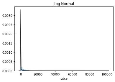
## 1) 总体分布概况（无界约翰逊分布等）
import scipy.stats as st
y = Train_data['price']
plt.figure(1); plt.title('Johnson SU')
sns.distplot(y, kde=False, fit=st.johnsonsu)
plt.figure(2); plt.title('Normal')
sns.distplot(y, kde=False, fit=st.norm)
plt.figure(3); plt.title('Log Normal')
sns.distplot(y, kde=False, fit=st.lognorm)

<matplotlib.axes._subplots.AxesSubplot at 0x1bd63b0bcc0>

在这里插入图片描述

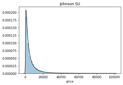
https://reference.wolfram.com/language/ref/JohnsonDistribution.html
具体来说，当观察到的分布为非正态分布，指数分布，逻辑分布时，通过双曲正弦变换将会分别生成对数正态的（ “SL” 类型），无界的（ “SU” 类型），有界的（“SB” 类型）Johnson 分布；而正态(“SN”)类型则对应于观察到的正态分布. 因为它的灵活性，Johnson 分布族被用来分析各种领域的实际的数据集，其中包括大气化学、生物医学工程、计量经济学、管理学和材料科学.

价格不服从正态分布，所以在进行回归之前，它必须进行转换。虽然对数变换做得很好，但最佳拟合是无界约翰逊分布

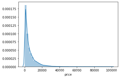
## 2) 查看skewness偏度 and kurtosis峰度
sns.distplot(Train_data['price']);
print("Skewness: %f" % Train_data['price'].skew())
print("Kurtosis: %f" % Train_data['price'].kurt())

Skewness: 3.346487
Kurtosis: 18.995183

在这里插入图片描述

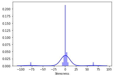
Train_data.skew(), Train_data.kurt()

(SaleID               6.017846e-17
 name                 5.576058e-01
 regDate              2.849508e-02
 model                1.484388e+00
 brand                1.150760e+00
 bodyType             9.915299e-01
 fuelType             1.595486e+00
 gearbox              1.317514e+00
 power                6.586318e+01
 kilometer           -1.525921e+00
 notRepairedDamage    2.430640e+00
 regionCode           6.888812e-01
 creatDate           -7.901331e+01
 price                3.346487e+00
 v_0                 -1.316712e+00
 v_1                  3.594543e-01
 v_2                  4.842556e+00
 v_3                  1.062920e-01
 v_4                  3.679890e-01
 v_5                 -4.737094e+00
 v_6                  3.680730e-01
 v_7                  5.130233e+00
 v_8                  2.046133e-01
 v_9                  4.195007e-01
 v_10                 2.522046e-02
 v_11                 3.029146e+00
 v_12                 3.653576e-01
 v_13                 2.679152e-01
 v_14                -1.186355e+00
 dtype: float64, SaleID                 -1.200000
 name                   -1.039945
 regDate                -0.697308
 model                   1.740483
 brand                   1.076201
 bodyType                0.206937
 fuelType                5.880049
 gearbox                -0.264161
 power                5733.451054
 kilometer               1.141934
 notRepairedDamage       3.908072
 regionCode             -0.340832
 creatDate            6881.080328
 price                  18.995183
 v_0                     3.993841
 v_1                    -1.753017
 v_2                    23.860591
 v_3                    -0.418006
 v_4                    -0.197295
 v_5                    22.934081
 v_6                    -1.742567
 v_7                    25.845489
 v_8                    -0.636225
 v_9                    -0.321491
 v_10                   -0.577935
 v_11                   12.568731
 v_12                    0.268937
 v_13                   -0.438274
 v_14                    2.393526
 dtype: float64)

sns.distplot(Train_data.skew(),color='blue',axlabel ='Skewness')

<matplotlib.axes._subplots.AxesSubplot at 0x1bd6453bf28>

在这里插入图片描述

sns.distplot(Train_data.kurt(),color='orange',axlabel ='Kurtness')

<matplotlib.axes._subplots.AxesSubplot at 0x1bd75f84c50>

在这里插入图片描述

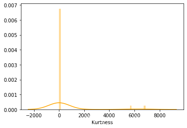
https://www.cnblogs.com/wyy1480/p/10474046.html
理解偏度和峰度，公式，不同值的含义。

## 3) 查看预测值的具体频数
plt.hist(Train_data['price'], orientation = 'vertical',histtype = 'bar', color ='red')
plt.show()

在这里插入图片描述

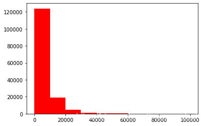
查看频数, 大于20000得值极少，其实这里也可以把这些当作特殊得值（异常值）直接用填充或者删掉，再前面进行

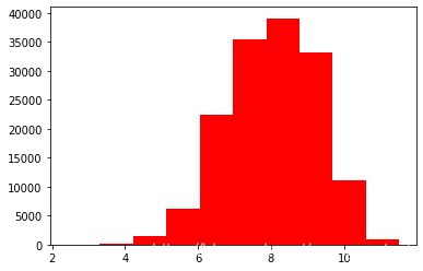
# log变换 z之后的分布较均匀，可以进行log变换进行预测，这也是预测问题常用的trick
plt.hist(np.log(Train_data['price']), orientation = 'vertical',histtype = 'bar', color ='red') 
plt.show()

在这里插入图片描述

特征分为类别特征和数字特征，并对类别特征查看unique分布

# 分离label即预测值
Y_train = Train_data['price']

# 这个区别方式适用于没有直接label coding的数据
# 这里不适用，需要人为根据实际含义来区分
# 数字特征
# numeric_features = Train_data.select_dtypes(include=[np.number])
# numeric_features.columns
# # 类型特征
# categorical_features = Train_data.select_dtypes(include=[np.object])
# categorical_features.columns

numeric_features = ['power', 'kilometer', 'v_0', 'v_1', 'v_2', 'v_3', 'v_4', 'v_5', 'v_6', 'v_7', 'v_8', 'v_9', 'v_10', 'v_11', 'v_12', 'v_13','v_14' ]

categorical_features = ['name', 'model', 'brand', 'bodyType', 'fuelType', 'gearbox', 'notRepairedDamage', 'regionCode',]

# 特征nunique分布
for cat_fea in categorical_features:
    print(cat_fea + "的特征分布如下：")
    print("{}特征有个{}不同的值".format(cat_fea, Train_data[cat_fea].nunique()))
    print(Train_data[cat_fea].value_counts())

name的特征分布如下：
name特征有个99662不同的值
708       282
387       282
55        280
1541      263
203       233
         ... 
5074        1
7123        1
11221       1
13270       1
174485      1
Name: name, Length: 99662, dtype: int64
model的特征分布如下：
model特征有个248不同的值
0.0      11762
19.0      9573
4.0       8445
1.0       6038
29.0      5186
         ...  
245.0        2
209.0        2
240.0        2
242.0        2
247.0        1
Name: model, Length: 248, dtype: int64
brand的特征分布如下：
brand特征有个40不同的值
0     31480
4     16737
14    16089
10    14249
1     13794
6     10217
9      7306
5      4665
13     3817
11     2945
3      2461
7      2361
16     2223
8      2077
25     2064
27     2053
21     1547
15     1458
19     1388
20     1236
12     1109
22     1085
26      966
30      940
17      913
24      772
28      649
32      592
29      406
37      333
2       321
31      318
18      316
36      228
34      227
33      218
23      186
35      180
38       65
39        9
Name: brand, dtype: int64
bodyType的特征分布如下：
bodyType特征有个8不同的值
0.0    41420
1.0    35272
2.0    30324
3.0    13491
4.0     9609
5.0     7607
6.0     6482
7.0     1289
Name: bodyType, dtype: int64
fuelType的特征分布如下：
fuelType特征有个7不同的值
0.0    91656
1.0    46991
2.0     2212
3.0      262
4.0      118
5.0       45
6.0       36
Name: fuelType, dtype: int64
gearbox的特征分布如下：
gearbox特征有个2不同的值
0.0    111623
1.0     32396
Name: gearbox, dtype: int64
notRepairedDamage的特征分布如下：
notRepairedDamage特征有个2不同的值
0.0    111361
1.0     14315
Name: notRepairedDamage, dtype: int64
regionCode的特征分布如下：
regionCode特征有个7905不同的值
419     369
764     258
125     137
176     136
462     134
       ... 
6414      1
7063      1
4239      1
5931      1
7267      1
Name: regionCode, Length: 7905, dtype: int64

# 特征nunique分布
for cat_fea in categorical_features:
    print(cat_fea + "的特征分布如下：")
    print("{}特征有个{}不同的值".format(cat_fea, Test_data[cat_fea].nunique()))
    print(Test_data[cat_fea].value_counts())

name的特征分布如下：
name特征有个37453不同的值
55       97
708      96
387      95
1541     88
713      74
         ..
22270     1
89855     1
42752     1
48899     1
11808     1
Name: name, Length: 37453, dtype: int64
model的特征分布如下：
model特征有个247不同的值
0.0      3896
19.0     3245
4.0      3007
1.0      1981
29.0     1742
         ... 
242.0       1
240.0       1
244.0       1
243.0       1
246.0       1
Name: model, Length: 247, dtype: int64
brand的特征分布如下：
brand特征有个40不同的值
0     10348
4      5763
14     5314
10     4766
1      4532
6      3502
9      2423
5      1569
13     1245
11      919
7       795
3       773
16      771
8       704
25      695
27      650
21      544
15      511
20      450
19      450
12      389
22      363
30      324
17      317
26      303
24      268
28      225
32      193
29      117
31      115
18      106
2       104
37       92
34       77
33       76
36       67
23       62
35       53
38       23
39        2
Name: brand, dtype: int64
bodyType的特征分布如下：
bodyType特征有个8不同的值
0.0    13985
1.0    11882
2.0     9900
3.0     4433
4.0     3303
5.0     2537
6.0     2116
7.0      431
Name: bodyType, dtype: int64
fuelType的特征分布如下：
fuelType特征有个7不同的值
0.0    30656
1.0    15544
2.0      774
3.0       72
4.0       37
6.0       14
5.0       10
Name: fuelType, dtype: int64
gearbox的特征分布如下：
gearbox特征有个2不同的值
0.0    37301
1.0    10789
Name: gearbox, dtype: int64
notRepairedDamage的特征分布如下：
notRepairedDamage特征有个2不同的值
0.0    37249
1.0     4720
Name: notRepairedDamage, dtype: int64
regionCode的特征分布如下：
regionCode特征有个6971不同的值
419     146
764      78
188      52
125      51
759      51
       ... 
7753      1
7463      1
7230      1
826       1
112       1
Name: regionCode, Length: 6971, dtype: int64

数字特征分析

numeric_features.append('price')

numeric_features

['power',
 'kilometer',
 'v_0',
 'v_1',
 'v_2',
 'v_3',
 'v_4',
 'v_5',
 'v_6',
 'v_7',
 'v_8',
 'v_9',
 'v_10',
 'v_11',
 'v_12',
 'v_13',
 'v_14',
 'price']

Train_data.head()

	SaleID	name	regDate	model	brand	bodyType	gearbox	power	kilometer	...	v_5	v_6	v_7	v_8	v_9	v_10	v_11	v_12	v_13	v_14
0	0	736	20040402	30.0	6	1.0	0.0	60	12.5	...	0.235676	0.101988	0.129549	0.022816	0.097462	-2.881803	2.804097	-2.420821	0.795292	0.914762
1	1	2262	20030301	40.0	1	2.0	0.0	0	15.0	...	0.264777	0.121004	0.135731	0.026597	0.020582	-4.900482	2.096338	-1.030483	-1.722674	0.245522
2	2	14874	20040403	115.0	15	1.0	0.0	163	12.5	...	0.251410	0.114912	0.165147	0.062173	0.027075	-4.846749	1.803559	1.565330	-0.832687	-0.229963
3	3	71865	19960908	109.0	10	0.0	1.0	193	15.0	...	0.274293	0.110300	0.121964	0.033395	0.000000	-4.509599	1.285940	-0.501868	-2.438353	-0.478699
4	4	111080	20120103	110.0	5	1.0	0.0	68	5.0	...	0.228036	0.073205	0.091880	0.078819	0.121534	-1.896240	0.910783	0.931110	2.834518	1.923482

5 rows × 29 columns

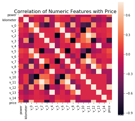
## 1) 相关性分析
price_numeric = Train_data[numeric_features]
correlation = price_numeric.corr()
print(correlation['price'].sort_values(ascending = False),'\n')

price        1.000000
v_12         0.692823
v_8          0.685798
v_0          0.628397
power        0.219834
v_5          0.164317
v_2          0.085322
v_6          0.068970
v_1          0.060914
v_14         0.035911
v_13        -0.013993
v_7         -0.053024
v_4         -0.147085
v_9         -0.206205
v_10        -0.246175
v_11        -0.275320
kilometer   -0.440519
v_3         -0.730946
Name: price, dtype: float64

f , ax = plt.subplots(figsize = (7, 7))

plt.title('Correlation of Numeric Features with Price',y=1,size=16)

sns.heatmap(correlation,square = True,  vmax=0.8)

<matplotlib.axes._subplots.AxesSubplot at 0x1bd653dc908>

在这里插入图片描述

del price_numeric['price']

## 2) 查看几个特征得 偏度和峰值
for col in numeric_features:
    print('{:15}'.format(col), 
          'Skewness: {:05.2f}'.format(Train_data[col].skew()) , 
          '   ' ,
          'Kurtosis: {:06.2f}'.format(Train_data[col].kurt())  
         )

power           Skewness: 65.86     Kurtosis: 5733.45
kilometer       Skewness: -1.53     Kurtosis: 001.14
v_0             Skewness: -1.32     Kurtosis: 003.99
v_1             Skewness: 00.36     Kurtosis: -01.75
v_2             Skewness: 04.84     Kurtosis: 023.86
v_3             Skewness: 00.11     Kurtosis: -00.42
v_4             Skewness: 00.37     Kurtosis: -00.20
v_5             Skewness: -4.74     Kurtosis: 022.93
v_6             Skewness: 00.37     Kurtosis: -01.74
v_7             Skewness: 05.13     Kurtosis: 025.85
v_8             Skewness: 00.20     Kurtosis: -00.64
v_9             Skewness: 00.42     Kurtosis: -00.32
v_10            Skewness: 00.03     Kurtosis: -00.58
v_11            Skewness: 03.03     Kurtosis: 012.57
v_12            Skewness: 00.37     Kurtosis: 000.27
v_13            Skewness: 00.27     Kurtosis: -00.44
v_14            Skewness: -1.19     Kurtosis: 002.39
price           Skewness: 03.35     Kurtosis: 019.00

## 3) 每个数字特征得分布可视化
f = pd.melt(Train_data, value_vars=numeric_features)
g = sns.FacetGrid(f, col="variable",  col_wrap=2, sharex=False, sharey=False)
g = g.map(sns.distplot, "value")

在这里插入图片描述

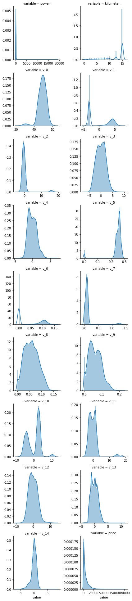
可以看到匿名特征相对分布均匀

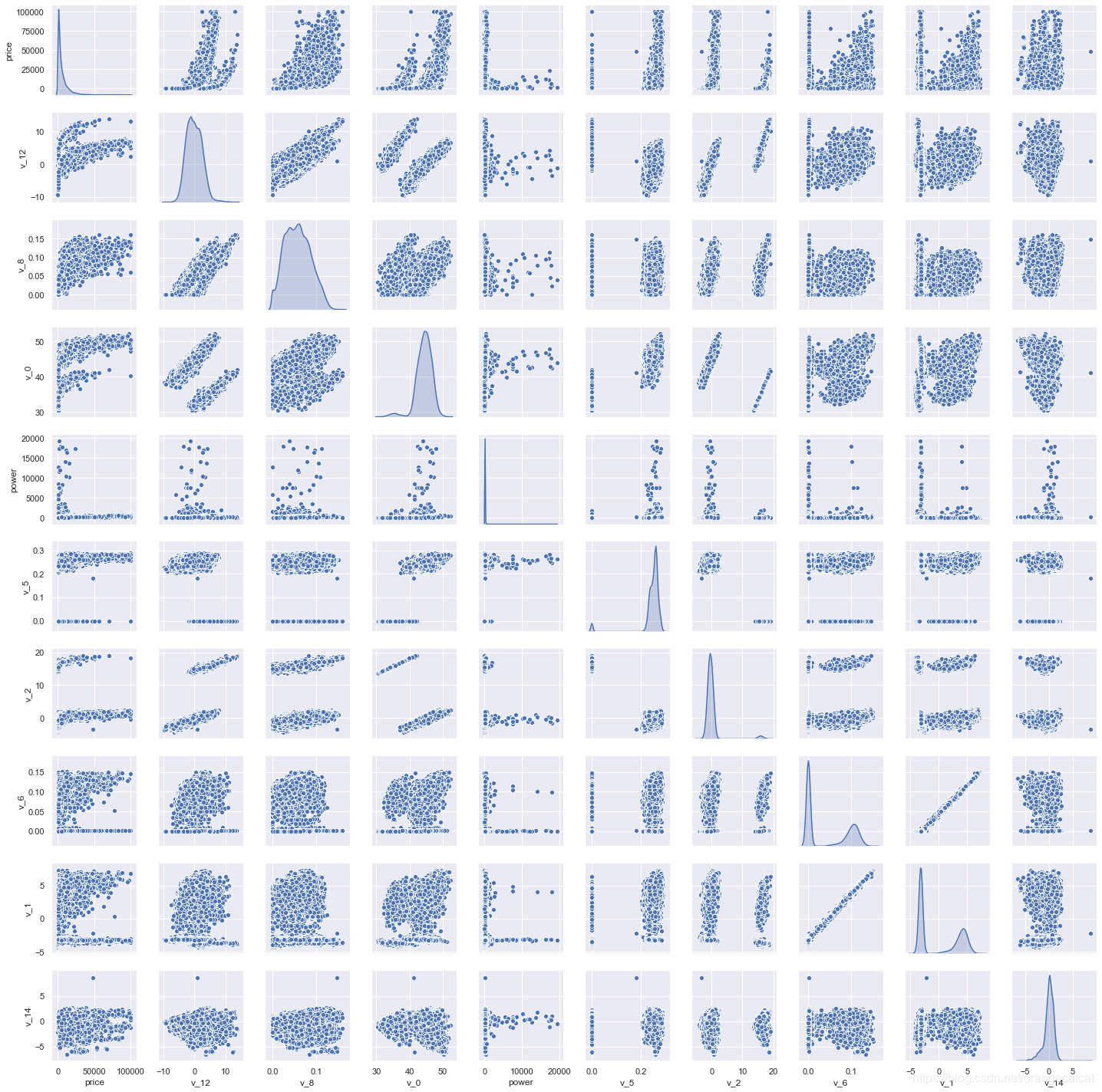
## 4) 数字特征相互之间的关系可视化
sns.set()
columns = ['price', 'v_12', 'v_8' , 'v_0', 'power', 'v_5',  'v_2', 'v_6', 'v_1', 'v_14']
sns.pairplot(Train_data[columns],size = 2 ,kind ='scatter',diag_kind='kde')
plt.show()

在这里插入图片描述

Train_data.columns

Index(['SaleID', 'name', 'regDate', 'model', 'brand', 'bodyType', 'fuelType',
       'gearbox', 'power', 'kilometer', 'notRepairedDamage', 'regionCode',
       'creatDate', 'price', 'v_0', 'v_1', 'v_2', 'v_3', 'v_4', 'v_5', 'v_6',
       'v_7', 'v_8', 'v_9', 'v_10', 'v_11', 'v_12', 'v_13', 'v_14'],
      dtype='object')

Y_train

0         1850
1         3600
2         6222
3         2400
4         5200
          ... 
149995    5900
149996    9500
149997    7500
149998    4999
149999    4700
Name: price, Length: 150000, dtype: int64

# https://www.jianshu.com/p/6e18d21a4cad 参考
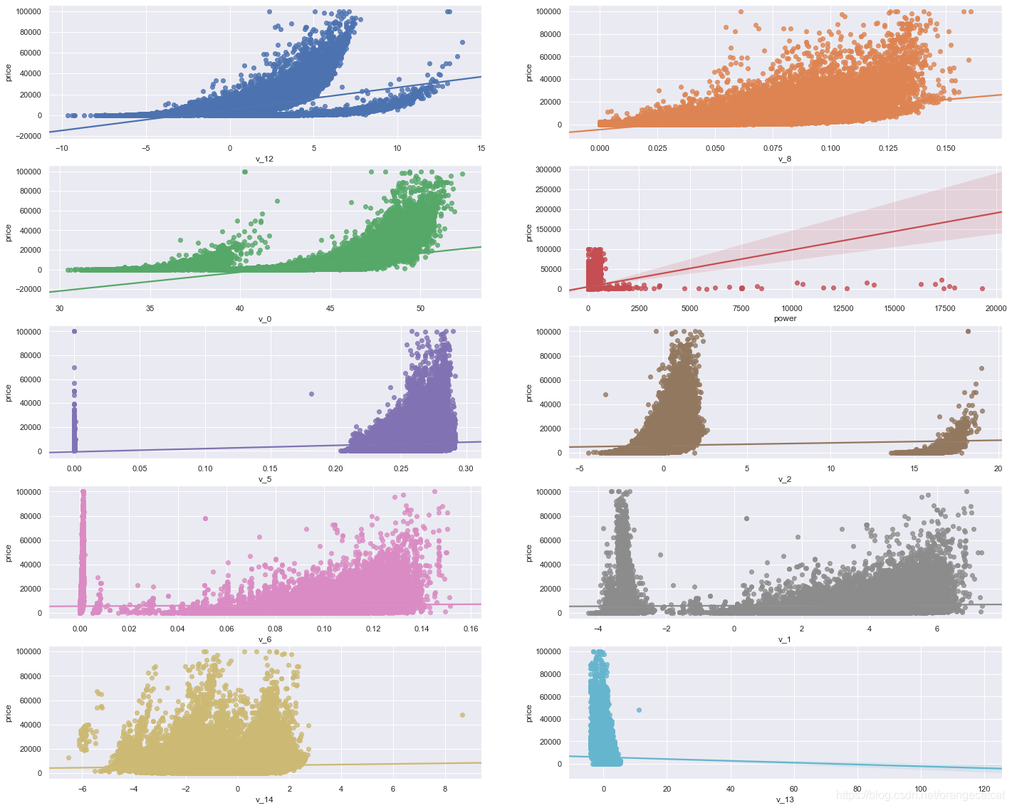
## 5) 多变量互相回归关系可视化
fig, ((ax1, ax2), (ax3, ax4), (ax5, ax6), (ax7, ax8), (ax9, ax10)) = plt.subplots(nrows=5, ncols=2, figsize=(24, 20))
# ['v_12', 'v_8' , 'v_0', 'power', 'v_5',  'v_2', 'v_6', 'v_1', 'v_14']
v_12_scatter_plot = pd.concat([Y_train,Train_data['v_12']],axis = 1)
sns.regplot(x='v_12',y = 'price', data = v_12_scatter_plot,scatter= True, fit_reg=True, ax=ax1)

v_8_scatter_plot = pd.concat([Y_train,Train_data['v_8']],axis = 1)
sns.regplot(x='v_8',y = 'price',data = v_8_scatter_plot,scatter= True, fit_reg=True, ax=ax2)

v_0_scatter_plot = pd.concat([Y_train,Train_data['v_0']],axis = 1)
sns.regplot(x='v_0',y = 'price',data = v_0_scatter_plot,scatter= True, fit_reg=True, ax=ax3)

power_scatter_plot = pd.concat([Y_train,Train_data['power']],axis = 1)
sns.regplot(x='power',y = 'price',data = power_scatter_plot,scatter= True, fit_reg=True, ax=ax4)

v_5_scatter_plot = pd.concat([Y_train,Train_data['v_5']],axis = 1)
sns.regplot(x='v_5',y = 'price',data = v_5_scatter_plot,scatter= True, fit_reg=True, ax=ax5)

v_2_scatter_plot = pd.concat([Y_train,Train_data['v_2']],axis = 1)
sns.regplot(x='v_2',y = 'price',data = v_2_scatter_plot,scatter= True, fit_reg=True, ax=ax6)

v_6_scatter_plot = pd.concat([Y_train,Train_data['v_6']],axis = 1)
sns.regplot(x='v_6',y = 'price',data = v_6_scatter_plot,scatter= True, fit_reg=True, ax=ax7)

v_1_scatter_plot = pd.concat([Y_train,Train_data['v_1']],axis = 1)
sns.regplot(x='v_1',y = 'price',data = v_1_scatter_plot,scatter= True, fit_reg=True, ax=ax8)

v_14_scatter_plot = pd.concat([Y_train,Train_data['v_14']],axis = 1)
sns.regplot(x='v_14',y = 'price',data = v_14_scatter_plot,scatter= True, fit_reg=True, ax=ax9)

v_13_scatter_plot = pd.concat([Y_train,Train_data['v_13']],axis = 1)
sns.regplot(x='v_13',y = 'price',data = v_13_scatter_plot,scatter= True, fit_reg=True, ax=ax10)

<matplotlib.axes._subplots.AxesSubplot at 0x1bd0387a5f8>

在这里插入图片描述

类别特征分析

## 1) unique分布
for fea in categorical_features:
    print(Train_data[fea].nunique())

categorical_features

['name',
 'model',
 'brand',
 'bodyType',
 'fuelType',
 'gearbox',
 'notRepairedDamage',
 'regionCode']

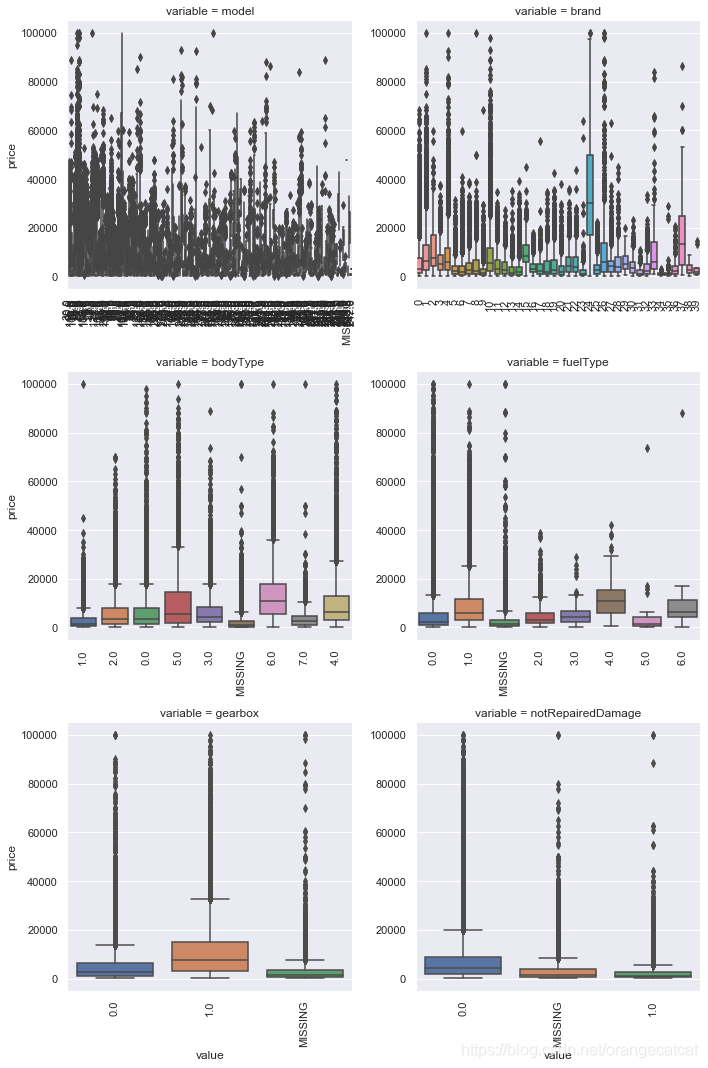
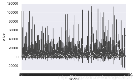
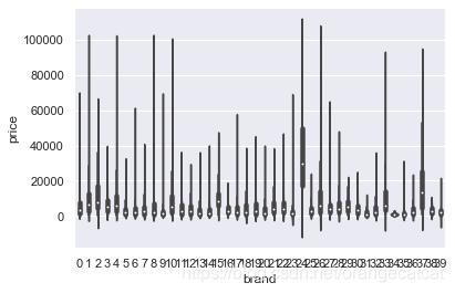
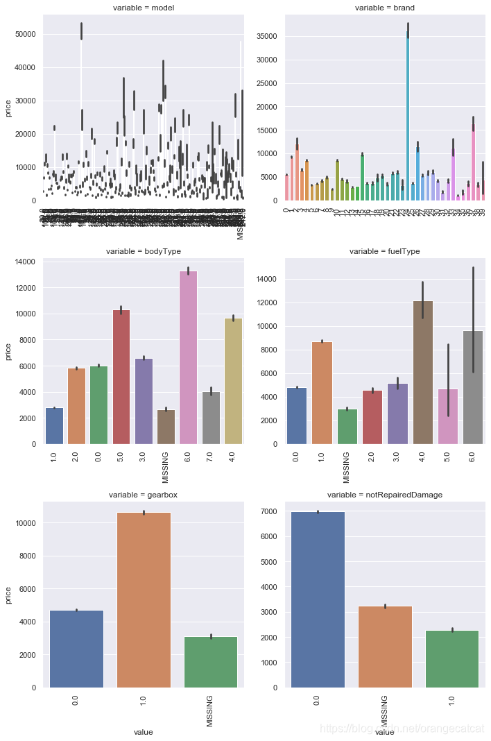
## 2) 类别特征箱形图可视化

# 因为 name和 regionCode的类别太稀疏了，这里我们把不稀疏的几类画一下
categorical_features = ['model',
 'brand',
 'bodyType',
 'fuelType',
 'gearbox',
 'notRepairedDamage']
for c in categorical_features:
    Train_data[c] = Train_data[c].astype('category')
    if Train_data[c].isnull().any():
        Train_data[c] = Train_data[c].cat.add_categories(['MISSING'])
        Train_data[c] = Train_data[c].fillna('MISSING')

def boxplot(x, y, **kwargs):
    sns.boxplot(x=x, y=y)
    x=plt.xticks(rotation=90)

f = pd.melt(Train_data, id_vars=['price'], value_vars=categorical_features)
g = sns.FacetGrid(f, col="variable",  col_wrap=2, sharex=False, sharey=False, size=5)
g = g.map(boxplot, "value", "price")

在这里插入图片描述

Train_data.columns

Index(['SaleID', 'name', 'regDate', 'model', 'brand', 'bodyType', 'fuelType',
       'gearbox', 'power', 'kilometer', 'notRepairedDamage', 'regionCode',
       'creatDate', 'price', 'v_0', 'v_1', 'v_2', 'v_3', 'v_4', 'v_5', 'v_6',
       'v_7', 'v_8', 'v_9', 'v_10', 'v_11', 'v_12', 'v_13', 'v_14'],
      dtype='object')

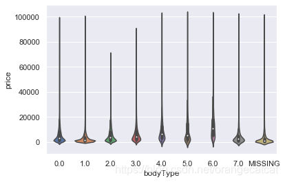
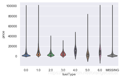
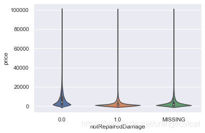
## 3) 类别特征的小提琴图可视化
catg_list = categorical_features
target = 'price'
for catg in catg_list :
    sns.violinplot(x=catg, y=target, data=Train_data)
    plt.show()

在这里插入图片描述

categorical_features = ['model',
 'brand',
 'bodyType',
 'fuelType',
 'gearbox',
 'notRepairedDamage']

## 4) 类别特征的柱形图可视化
def bar_plot(x, y, **kwargs):
    sns.barplot(x=x, y=y)
    x=plt.xticks(rotation=90)

f = pd.melt(Train_data, id_vars=['price'], value_vars=categorical_features)
g = sns.FacetGrid(f, col="variable",  col_wrap=2, sharex=False, sharey=False, size=5)
g = g.map(bar_plot, "value", "price")

在这里插入图片描述

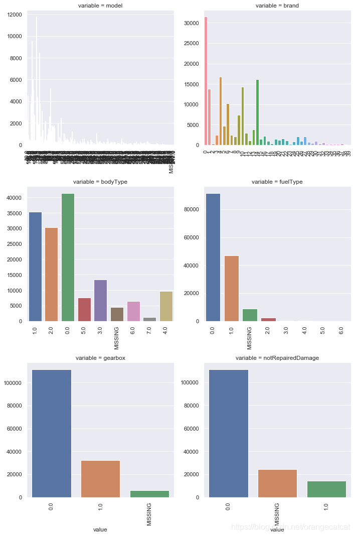
##  5) 类别特征的每个类别频数可视化(count_plot)
def count_plot(x,  **kwargs):
    sns.countplot(x=x)
    x=plt.xticks(rotation=90)

f = pd.melt(Train_data,  value_vars=categorical_features)
g = sns.FacetGrid(f, col="variable",  col_wrap=2, sharex=False, sharey=False, size=5)
g = g.map(count_plot, "value")

在这里插入图片描述

用pandas_profiling生成数据报告

import pandas_profiling

pfr = pandas_profiling.ProfileReport(Train_data)
pfr.to_file("./example.html")

HBox(children=(FloatProgress(value=0.0, description='variables', max=29.0, style=ProgressStyle(description_wid…






HBox(children=(FloatProgress(value=0.0, description='correlations', max=6.0, style=ProgressStyle(description_w…






HBox(children=(FloatProgress(value=0.0, description='interactions [continuous]', max=529.0, style=ProgressStyl…






HBox(children=(FloatProgress(value=0.0, description='table', max=1.0, style=ProgressStyle(description_width='i…






HBox(children=(FloatProgress(value=0.0, description='missing', max=2.0, style=ProgressStyle(description_width=…






HBox(children=(FloatProgress(value=0.0, description='warnings', max=3.0, style=ProgressStyle(description_width…






HBox(children=(FloatProgress(value=0.0, description='package', max=1.0, style=ProgressStyle(description_width=…






HBox(children=(FloatProgress(value=0.0, description='build report structure', max=1.0, style=ProgressStyle(des…

from: https://github.com/datawhalechina/team-learning/blob/master/%E6%95%B0%E6%8D%AE%E6%8C%96%E6%8E%98%E5%AE%9E%E8%B7%B5%EF%BC%88%E4%BA%8C%E6%89%8B%E8%BD%A6%E4%BB%B7%E6%A0%BC%E9%A2%84%E6%B5%8B%EF%BC%89/Task2%20%E6%95%B0%E6%8D%AE%E5%88%86%E6%9E%90.md
数据探索有利于我们发现数据的一些特性，数据之间的关联性，对于后续的特征构建是很有帮助的。

对于数据的初步分析（直接查看数据，或.sum(), .mean()，.descirbe()等统计函数）可以从：样本数量，训练集数量，是否有时间特征，是否是时许问题，特征所表示的含义（非匿名特征），特征类型（字符类似，int，float，time），特征的缺失情况（注意缺失的在数据中的表现形式，有些是空的有些是”NAN”符号等），特征的均值方差情况。

分析记录某些特征值缺失占比30%以上样本的缺失处理，有助于后续的模型验证和调节，分析特征应该是填充（填充方式是什么，均值填充，0填充，众数填充等），还是舍去，还是先做样本分类用不同的特征模型去预测。

对于异常值做专门的分析，分析特征异常的label是否为异常值（或者偏离均值较远或者事特殊符号）,异常值是否应该剔除，还是用正常值填充，是记录异常，还是机器本身异常等。

对于Label做专门的分析，分析标签的分布情况等。

进步分析可以通过对特征作图，特征和label联合做图（统计图，离散图），直观了解特征的分布情况，通过这一步也可以发现数据之中的一些异常值等，通过箱型图分析一些特征值的偏离情况，对于特征和特征联合作图，对于特征和label联合作图，分析其中的一些关联性。
x=plt.xticks(rotation=90)

f = pd.melt(Train_data, id_vars=[‘price’], value_vars=categorical_features)
g = sns.FacetGrid(f, col=“variable”, col_wrap=2, sharex=False, sharey=False, size=5)
g = g.map(bar_plot, “value”, “price”)



[外链图片转存中...(img-iI6CyuLE-1585041548470)]



```python
##  5) 类别特征的每个类别频数可视化(count_plot)
def count_plot(x,  **kwargs):
    sns.countplot(x=x)
    x=plt.xticks(rotation=90)

f = pd.melt(Train_data,  value_vars=categorical_features)
g = sns.FacetGrid(f, col="variable",  col_wrap=2, sharex=False, sharey=False, size=5)
g = g.map(count_plot, "value")

[外链图片转存中…(img-sFAFAAHd-1585041548470)]

用pandas_profiling生成数据报告

import pandas_profiling

pfr = pandas_profiling.ProfileReport(Train_data)
pfr.to_file("./example.html")

HBox(children=(FloatProgress(value=0.0, description='variables', max=29.0, style=ProgressStyle(description_wid…






HBox(children=(FloatProgress(value=0.0, description='correlations', max=6.0, style=ProgressStyle(description_w…






HBox(children=(FloatProgress(value=0.0, description='interactions [continuous]', max=529.0, style=ProgressStyl…






HBox(children=(FloatProgress(value=0.0, description='table', max=1.0, style=ProgressStyle(description_width='i…






HBox(children=(FloatProgress(value=0.0, description='missing', max=2.0, style=ProgressStyle(description_width=…






HBox(children=(FloatProgress(value=0.0, description='warnings', max=3.0, style=ProgressStyle(description_width…






HBox(children=(FloatProgress(value=0.0, description='package', max=1.0, style=ProgressStyle(description_width=…






HBox(children=(FloatProgress(value=0.0, description='build report structure', max=1.0, style=ProgressStyle(des…

对于Label做专门的分析，分析标签的分布情况等。

进步分析可以通过对特征作图，特征和label联合做图（统计图，离散图），直观了解特征的分布情况，通过这一步也可以发现数据之中的一些异常值等，通过箱型图分析一些特征值的偏离情况，对于特征和特征联合作图，对于特征和label联合作图，分析其中的一些关联性。

orangecatcat

关注

0
点赞
踩
2

收藏

觉得还不错? 一键收藏
0
评论
Task2-探索性数据分析(EDA, Exploratory Data Analysis)

1. 为什么要进行EDA初步从数据中得到一些简单、直观的信息，加强对题目、数据本身的理解，为进一步分析比如特征做铺垫。2. EAD会做些什么一些常用的库：pandas, numpy, scipy, matplotlib, seabon在看数据前，导入数据（需相应的库）（1）宏观角度认识数据head(), shapedescribe()info()缺失值异常值（2）一些统计特征...
复制链接

扫一扫