


一、像差的概念:
像差是指光学系统中的成像缺陷。几何光学上把像差(几何像差)分为单色光像差和色光像差,前者包括球差、彗差、像散、场曲和畸变,后者包括位置色差和倍率色差;而物理光学上把像差称之为波前像差或波阵面像差,即是点光源发出的球面波经光学系统后形成的波形与理想球面波之间的距离。波前像差可以通过Zernike多项式周期表或球差、彗差等几何像差来表达。1、球差是指轴上点光源发出的光线经屈光系统后,近轴光线与边缘光线像点之间的距离。存在球差的光学系统所形成的像是对称的弥散圆。

2、彗差是指轴外点光源发出的光线经屈光系统后,上光线和下光线的交点离开主光线的距离。存在彗差的光学系统形成的像是不对称的弥散斑。

3、像散是子午面上的像点和弧矢面上的像点的距离。子午面为通过光轴的平面,而弧矢面为垂直于子午面并通过主光线的平面。
4、场曲为平面物体通过光学系统后形成的矢状弯曲。人眼的视网膜是球形向后弯曲状,正好能补偿眼屈光系统产生的这种成像缺陷。
5、畸变为方形物体通过光学系统后周边各点产生了不同棱镜像移所致。

6、位置色差即轴位色差,白光中不同波长的光线经光学系统后形成像点的距离,短波长的交点近于长波长的交点。
7、倍率色差某一物体经光学系统成像后不同波长的光线在物像大小上的差异。
人眼是一复杂的光学系统,存在波前像差。波前像差分为低阶像差和高阶像差。按照Zernike多项式周期表,1-2阶为低阶像差,3阶以上为高阶像差。屈光不正属于低阶像差。
二、像差产生的原因:
人眼产生像差的原因包括各屈光面固有的成像缺陷、调节时的动态变化和各屈光面间的相互影响等多方面。1、角膜角膜前表面不是理想的球面,而是非球面,然而中央4毫米区域却近似球形,所以产生球差。角膜顶点处较陡,边缘部较扁平。但顶点并不总在角膜的几何中心,往往偏下,不规则角膜的顶点偏离几何中心可达2mm以上。角膜各部分的厚度和曲率半径在各测量点上并不一致,这些就是角膜的不对称性和表面不规则性。
2、晶状体晶状体前表面较平坦,可抵消80%的角膜球差,但晶状体前表面也不平滑。随年龄增加,晶状体增厚,核发生硬化,各部位屈光指数不一致。晶状体的调节变化,除晶状体屈光力发生改变外,还可有X、Y、Z轴的变化。晶状体亦存在不对称性和表面不规则性。
3、其他玻璃体的变性、液化、混浊、后脱离等。泪膜的不均匀和不稳定,如干眼症或用药等影响。房水的改变。高度近视患者的视网膜形态变化等。
4、角膜和晶状体的光学中心不一致;与入瞳中心不一致。
5、光轴和视轴本身的偏差。
6、瞳孔除随光线的强弱发生改变,人群中存在相当大的生理差异。瞳孔增大,像差明显增加。入瞳中心并不在角膜的几何中心的对应点上。
三、Zernike多项式与Zernike矩
3.1 Zernike多项式
以下内容大部分摘自:http://blog.csdn.net/wrj19860202/article/details/6334275
Zernike在1934年引入了一组定义在单位圆 上的复值函数集{
 },{
},{ }具有完备性和正交性,使得它可以表示定义在单位圆盘内的任何平方可积函数。其定义为:
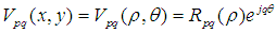
 表示原点到点
 的矢量长度;
 表示矢量
表示矢量 与
与 轴逆时针方向的夹角,
 是实值径向多项式:
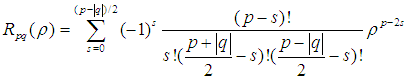
称为Zernike多项式,Zernike多项式满足正交性:

 为克罗内克符号,

 是
是 的共轭多项式,由于Zernike多项式的正交完备性,所以在单位圆内的任何图像
 都可以唯一的用下面式子来展开:
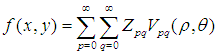
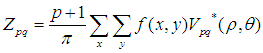
式子中 就是Zernike矩,其定义为:
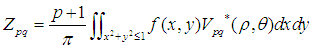
式子中 和
和 采用的是不同的坐标系,
 采用直角坐标,而
 采用的极坐标系,在计算的时候要进行坐标转换。对于离散的数字图像,可将积分形式改为累加形式:
 ,
, 
Noll index ( ) ) | Radial degree ( ) ) | Azimuthal degree ( ) ) |  | Classical name |
|---|---|---|---|---|
| 1 | 0 | 0 |  | Piston |
| 2 | 1 | 1 |  | Tip (lateral position) (X-Tilt) |
| 3 | 1 | −1 |  | Tilt (lateral position) (Y-Tilt) |
| 4 | 2 | 0 |  | Defocus (longitudinal position) |
| 5 | 2 | −2 |  | Oblique astigmatism |
| 6 | 2 | 2 |  | Vertical astigmatism |
| 7 | 3 | −1 |  | Vertical coma |
| 8 | 3 | 1 |  | Horizontal coma |
| 9 | 3 | −3 |  | Vertical trefoil |
| 10 | 3 | 3 |  | Oblique trefoil |
| 11 | 4 | 0 |  | Primary spherical |
| 12 | 4 | 2 |  | Vertical secondary astigmatism |
| 13 | 4 | −2 |  | Oblique secondary astigmatism |
| 14 | 4 | 4 |  | Oblique quadrafoil |
| 15 | 4 | −4 |  | Vertical quadrafoil |
通常使用幂级数展开式的形式来描述光学系统的像差。由于泽尼克多项式和光学检测中观测到的像差多项式的形式是一致的,因而常用zernike描述波前特性。但并不意味着泽尼克多项式就是用来拟合检测数据的最佳多项式形式。在某些情况下,用泽尼克多项式来描述波前数据具有很大的局限性。例如,当需要考虑空气扰动的时候,泽尼克多项式几乎没有什么价值。同样地,我们也无法找到一组合适的泽尼克多项式来描述单点金刚石车削加工(single point diamond turning process)中的制造误差。为了准确地描述圆锥面光学元件(conical optical elements)的对准误差,必须对泽尼克多项式进行修正。盲目地使用泽尼克多项式来表达检测数据只会导致糟糕的结果。
泽尼克多项式是由无穷数量的多项式完全集组成的,它有两个变量,ρ和θ,它在单位圆内部是连续正交的。需要注意的是,泽尼克多项式仅在单位圆的内部连续区域是正交的,通常在单位圆内部的离散的坐标上是不具备正交性质的。泽尼克多项式具有三个和其他正交多项式集不一样的性质。
1.泽尼克多项式Z(ρ, θ)可以被化解为径向坐标ρ和角度坐标θ的函数,其形式如下: Z (ρ, θ) = R ( ρ ) G ( θ ), 这里,关于角度的函数G(θ)是一个以2π弧度为周期的连续函数,并且满足当坐标系旋转α角度之后,其形式不发生改变,也就是旋转不变性。
2.泽尼克多项式的第二个性质是径向函数R ( ρ ) (Radial Function)必须是ρ的n次多项式,并且不包含幂次低于m次的ρ方项。
3.第三个性质是当m为偶数时R(ρ)也为偶函数,m为奇数时,R(ρ)也为奇函数。 径向多项式R ( ρ )可以看作是雅可比多项式(Jacobi polynomials)的特例
3.2 矩的概念
图像识别的一个核心问题是图像的特征提取,即用一组简单的数据来描述整个图像,这组数据越简单越有代表性越好。良好的特征不受光线、噪点、几何形变的干扰,图像不变矩就是其中一个。矩是概率与统计中的一个概念,是随机变量的一种数字特征。设x为随机变量,c为常数,k为正整数。则
1. c=0时表示x的k阶原点矩.
2. c=E(x)时表示x的k阶中心矩。
一阶原点矩就是期望。一阶中心矩μ1=0,二阶中心矩μ2就是X的方差Var(X)。在统计学上,高于4阶的矩极少使用。μ3可以去衡量分布是否有偏。μ4可以去衡量分布(密度)在均值附近的陡峭程度如何。
针对于一幅图像,我们把像素的坐标看成是一个二维随机变量(X,Y),那么一幅灰度图像可以用二维灰度密度函数来表示,因此可以用矩来描述灰度图像的特征。
不变矩(Invariant Moments)是一处高度浓缩的图像特征,具有平移、灰度、尺度、旋转不变性。M.K.Hu在1961年首先提出了不变矩的概念。1979年M.R.Teague根据正交多项式理论提出了Zernike矩。
3.3 Zernike矩
计算一副图像的Zernike矩时,必须将图像的中心移到坐标的原点,将图像的像素点映射到单位圆内,由于Zernike矩具有旋转不变性,可以将 作为图像的不变特征,其中图像的低频特征有p值小的
 提取,高频特征由p值高的
 提取。Zernike矩可以构造任意高阶矩,由于Zernike矩只具有旋转不变性,不具有平移和尺度不变性,所以要提前对图像进行归一化,采用标准矩的方法来归一化一副图像,标准矩定义为:
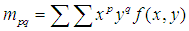 ,由标准矩我们可以得到图像的"重心",


我们将图像的"重心"移动到单位圆的圆心(即坐标的原点),便解决了平移问题。 表征了图像的"面积",归一图像的尺度无非就是把他们的大小变为一致的,(这里的大小指的是图像目标物的大小,不是整幅图像的大小,"面积"也是目标物的"面积")。
所以,对图像进行变换![]() 就可以达到图像尺寸一致的目的。
就可以达到图像尺寸一致的目的。
综合上面结果,对图像进行 变换,最终图像
 的Zernike矩就是平移,尺寸和旋转不变的。
3.4 实例程序:matlab
function z = zernfun(n,m,r,theta,nflag)
%ZERNFUN Zernike functions of order N and frequency M on the unit circle.
%   Z = ZERNFUN(N,M,R,THETA) returns the Zernike functions of order N
%   and angular frequency M, evaluated at positions (R,THETA) on the
%   unit circle.  N is a vector of positive integers (including 0), and
%   M is a vector with the same number of elements as N.  Each element
%   k of M must be a positive integer, with possible values M(k) = -N(k)
%   to +N(k) in steps of 2.  R is a vector of numbers between 0 and 1,
%   and THETA is a vector of angles.  R and THETA must have the same
%   length.  The output Z is a matrix with one column for every (N,M)
%   pair, and one row for every (R,THETA) pair.
%
%   Z = ZERNFUN(N,M,R,THETA,'norm') returns the normalized Zernike
%   functions.  The normalization factor sqrt((2-delta(m,0))*(n+1)/pi),
%   with delta(m,0) the Kronecker delta, is chosen so that the integral
%   of (r * [Znm(r,theta)]^2) over the unit circle (from r=0 to r=1,
%   and theta=0 to theta=2*pi) is unity.  For the non-normalized
%   polynomials, max(Znm(r=1,theta))=1 for all [n,m].
%
%   The Zernike functions are an orthogonal basis on the unit circle.
%   They are used in disciplines such as astronomy, optics, and
%   optometry to describe functions on a circular domain.
%
%   The following table lists the first 15 Zernike functions.
%
%       n    m    Zernike function             Normalization
%       ----------------------------------------------------
%       0    0    1                              1/sqrt(pi)
%       1    1    r * cos(theta)                 2/sqrt(pi)
%       1   -1    r * sin(theta)                 2/sqrt(pi)
%       2    2    r^2 * cos(2*theta)             sqrt(6/pi)
%       2    0    (2*r^2 - 1)                    sqrt(3/pi)
%       2   -2    r^2 * sin(2*theta)             sqrt(6/pi)
%       3    3    r^3 * cos(3*theta)             sqrt(8/pi)
%       3    1    (3*r^3 - 2*r) * cos(theta)     sqrt(8/pi)
%       3   -1    (3*r^3 - 2*r) * sin(theta)     sqrt(8/pi)
%       3   -3    r^3 * sin(3*theta)             sqrt(8/pi)
%       4    4    r^4 * cos(4*theta)             sqrt(10/pi)
%       4    2    (4*r^4 - 3*r^2) * cos(2*theta) sqrt(10/pi)
%       4    0    6*r^4 - 6*r^2 + 1              sqrt(5/pi)
%       4   -2    (4*r^4 - 3*r^2) * sin(2*theta) sqrt(10/pi)
%       4   -4    r^4 * sin(4*theta)             sqrt(10/pi)
%       ----------------------------------------------------
%
%   Example 1:
%
%       % Display the Zernike function Z(n=5,m=1)
%       x = -1:0.01:1;
%       [X,Y] = meshgrid(x,x);
%       [theta,r] = cart2pol(X,Y);
%       idx = r<=1;
%       z = nan(size(X));
%       z(idx) = zernfun(5,1,r(idx),theta(idx));
%       figure
%       pcolor(x,x,z), shading interp
%       axis square, colorbar
%       title('Zernike function Z_5^1(r,\theta)')
%
%   Example 2:
%
%       % Display the first 10 Zernike functions
%       x = -1:0.01:1;
%       [X,Y] = meshgrid(x,x);
%       [theta,r] = cart2pol(X,Y);
%       idx = r<=1;
%       z = nan(size(X));
%       n = [0  1  1  2  2  2  3  3  3  3];
%       m = [0 -1  1 -2  0  2 -3 -1  1  3];
%       Nplot = [4 10 12 16 18 20 22 24 26 28];
%       y = zernfun(n,m,r(idx),theta(idx));
%       figure('Units','normalized')
%       for k = 1:10
%           z(idx) = y(:,k);
%           subplot(4,7,Nplot(k))
%           pcolor(x,x,z), shading interp
%           set(gca,'XTick',[],'YTick',[])
%           axis square
%           title(['Z_{' num2str(n(k)) '}^{' num2str(m(k)) '}'])
%       end
%
%   See also ZERNPOL, ZERNFUN2.

%   Paul Fricker 2/28/2012

% Check and prepare the inputs:
% -----------------------------
if ( ~any(size(n)==1) ) || ( ~any(size(m)==1) )
    error('zernfun:NMvectors','N and M must be vectors.')
end

if length(n)~=length(m)
    error('zernfun:NMlength','N and M must be the same length.')
end

n = n(:);
m = m(:);
if any(mod(n-m,2))
    error('zernfun:NMmultiplesof2', ...
          'All N and M must differ by multiples of 2 (including 0).')
end

if any(m>n)
    error('zernfun:MlessthanN', ...
          'Each M must be less than or equal to its corresponding N.')
end

if any( r>1 | r<0 )
    error('zernfun:Rlessthan1','All R must be between 0 and 1.')
end

if ( ~any(size(r)==1) ) || ( ~any(size(theta)==1) )
    error('zernfun:RTHvector','R and THETA must be vectors.')
end

r = r(:);
theta = theta(:);
length_r = length(r);
if length_r~=length(theta)
    error('zernfun:RTHlength', ...
          'The number of R- and THETA-values must be equal.')
end

% Check normalization:
% --------------------
if nargin==5 && ischar(nflag)
    isnorm = strcmpi(nflag,'norm');
    if ~isnorm
        error('zernfun:normalization','Unrecognized normalization flag.')
    end
else
    isnorm = false;
end

%%%%%%%%%%%%%%%%%%%%%%%%%%%%%%%%%%%%%%%%%%%%
% Compute the Zernike Polynomials
%%%%%%%%%%%%%%%%%%%%%%%%%%%%%%%%%%%%%%%%%%%%

% Determine the required powers of r:
% -----------------------------------
m_abs = abs(m);
rpowers = [];
for j = 1:length(n)
    rpowers = [rpowers m_abs(j):2:n(j)];
end
rpowers = unique(rpowers);

% Pre-compute the values of r raised to the required powers,
% and compile them in a matrix:
% -----------------------------
if rpowers(1)==0
    rpowern = arrayfun(@(p)r.^p,rpowers(2:end),'UniformOutput',false);
    rpowern = cat(2,rpowern{:});
    rpowern = [ones(length_r,1) rpowern];
else
    rpowern = arrayfun(@(p)r.^p,rpowers,'UniformOutput',false);
    rpowern = cat(2,rpowern{:});
end

% Compute the values of the polynomials:
% --------------------------------------
z = zeros(length_r,length(n));
for j = 1:length(n)
    s = 0:(n(j)-m_abs(j))/2;
    pows = n(j):-2:m_abs(j);
    for k = length(s):-1:1
        p = (1-2*mod(s(k),2))* ...
                   prod(2:(n(j)-s(k)))/              ...
                   prod(2:s(k))/                     ...
                   prod(2:((n(j)-m_abs(j))/2-s(k)))/ ...
                   prod(2:((n(j)+m_abs(j))/2-s(k)));
        idx = (pows(k)==rpowers);
        z(:,j) = z(:,j) + p*rpowern(:,idx);
    end

    if isnorm
        z(:,j) = z(:,j)*sqrt((1+(m(j)~=0))*(n(j)+1)/pi);
    end
end
% END: Compute the Zernike Polynomials
%%%%%%%%%%%%%%%%%%%%%%%%%%%%%%%%%%%%%%%%%%%%

% Compute the Zernike functions:
% ------------------------------
idx_pos = m>0;
idx_neg = m<0;

if any(idx_pos)
    z(:,idx_pos) = z(:,idx_pos).*cos(theta*m_abs(idx_pos)');
end
if any(idx_neg)
    z(:,idx_neg) = z(:,idx_neg).*sin(theta*m_abs(idx_neg)');
end
% Display the Zernike function Z(n=5,m=1)
clc,clear all,close all;
x = -1:0.01:1;
[X,Y] = meshgrid(x,x);
[theta,r] = cart2pol(X,Y);
idx = r<=1;
z = nan(size(X));
z(idx) = zernfun(5,1,r(idx),theta(idx));
figure
pcolor(x,x,z), shading interp
axis square,  colorbar
title('Zernike function Z_5^1(r,\theta)')
参考:
http://changzhengdr.blog.sohu.com/108180288.html
http://download.csdn.net/detail/piaoxuezhong/9791297
https://wenku.baidu.com/view/4576361614791711cc791761.html
http://blog.csdn.net/wrj19860202/article/details/6334275
http://www.opt.indiana.edu/vsg/library/vsia/vsia-2000_taskforce/TOPS4_2.html


 773
773

 被折叠的 条评论
为什么被折叠?
被折叠的 条评论
为什么被折叠?
 到【灌水乐园】发言


