


在http://write.blog.csdn.net/postedit/78212814中介绍了同态滤波算法,本片继续总结retinex算法,不过开始之前先介绍一下色彩恒常性的概念:
色彩恒常性
在人体生物学领域中,颜色恒常性是指当照射物体表面的颜色光发生变化时,人们对该物体表面颜色的知觉仍然保持不变的知觉特性。
Retinex算法
Retinex这个词是由视网膜(Retina)和大脑皮层(Cortex)两个词组合构成的,Retinex 理论的基本内容是:(1)物体的颜色是由物体对长波(红)、中波(绿)和短波(蓝)光线的反射能力决定的,而不是由反射光强度的绝对值决定的;(2)物体的色彩不受光照非均性的影响,具有一致性,即Retinex理论是以色感一致性(颜色恒常性)为基础的。
如下图所示,观察者所看到的物体的图像S是由物体表面对入射光L反射得到的,反射率R由物体本身决定,不受入射光L变化。
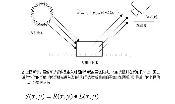
Retinex理论的基本假设是原始图像S是光照图像L和反射率图像R的乘积,即可表示为下式的形式:
![]()
基于Retinex的图像增强的目的就是从原始图像S中估计出光照L,从而分解出R,消除光照不均的影响,以改善图像的视觉效果。在处理中,通常将图像转至对数域,将乘积关系转换为和的关系:
![clip_image008[4]](http://img.2cto.com/2016/0702/20160702091545470.png "clip_image008[4]")
Retinex方法的核心就是估测照度L,从图像S中估测L分量,并去除L分量,得到原始反射分量R,即:
![clip_image010[4]](http://img.2cto.com/2016/0702/20160702091545772.png "clip_image010[4]")
函数f(s)实现对照度L的估计。按照发展历程将 Retinex 算法分成 3 类:
(2)迭代Retinex算法是一种迭代形式的Retinex算法,由Frankle和Mccann提出,也称多分辨率 Retinex 算法, 采用矩阵计算代替路径计算, 在路径计算中,依次将像素添加到路径中,以串行方式比较像素值 ,根据路径的长度确定距离函数;而在矩阵计算中, 比值和乘积运算可并行处理, 根据迭代次数确定距离函数。迭代Retinex算法的问题是参数的不确定性 , 参数的选取对最终结果起决定性作用。
(3)基于邻域的Retinex算法的理论基础为照度分量的强度一般变化缓慢, 在频域中表现为低频成分,而不同物体表面材质的反射率差异较大, 表现为高频成分。算法采用低通滤波的方法估计照度分量 , 也称为中心/邻域 ( center/suround )Retinex算法。对于图像中的各像素 ,计算该像素值与邻域内像 素加权值的非线性比值 ,即为该像素的新像素值,通过平滑函数的空域卷积获得邻域内像素的加权值 , 权重由平滑函数的系数给出。Jobson 等人对使用不同类型平滑函数的算法性能进行了评价 , 由此确定了高斯函数 , 提出单尺度 Retinex(SSR )算法 ,并将其扩展到多尺度, 多尺度 Retinex(MsR )算法是计算不同尺度的3幅SSR 图像的平均值。
经典算法容易出现光晕,对于照度估计和去除光晕等问题后来有基于Retinex的改进算法,这里暂不介绍,下面介绍SFU Computational Vision Lab公开的两种经典算法:McCann Retinex和McCann99 Retinex算法,以及基于邻域的几种Retinex算法。这里我基本是参照了参考2中说法。
McCann Retinex算法

Frankle-McCann算法使用如上图所示的螺旋结构的路径用于像素间的比较,这种路径选择包含了整个图像的全局明暗关系,越靠近预测中心点选取的点数越多,因为靠的近的像素点与中心像素点的相关性要比远处的高。具体操作可以参照程序:
该算法估测图像经过以下几个步骤(参考2):
1. 将原图像变换到对数域S;
2. 初始化常数图像矩阵R,作为迭代运算的初始值;
3. 计算路径,如上图所示,从远到近排列;
4. 对路径上的像素点按照如下公式运算:
![clip_image010[8]](http://images.cnitblog.com/blog/616589/201404/201552474167808.png "clip_image010[8]")
![]()
公式所表示的大致意思为:从远到近,中心点像素值减去路径上的像素值得到的差值的一半与前一时刻的估计值之间的和。最终,中心像素点的像素大致的形式为
![clip_image014[6]](http://images.cnitblog.com/blog/616589/201404/201552522138476.png "clip_image014[6]")
1.按照程序里的实现,路径选择像素数的确定值shift是指小于图像行或列较小值的2的最大指数倍-1,好绕口~请参见程序里的shift的定义方式。
2.CompareWith(,)函数按照步骤4的运算方式对像素点的亮度进行估计。
3.迭代次数我测试函数里设的10,这个一般要大于3吧,可以根据测试结果多尝试一下,以便增强效果。
下面是matlab函数实现:
function Retinex = retinex_frankle_mccann(L, nIterations)

% RETINEX_FRANKLE_McCANN:
%         Computes the raw Retinex output from an intensity image, based on the
%         original model described in:
%         Frankle, J. and McCann, J., "Method and Apparatus for Lightness Imaging"
%         US Patent #4,384,336, May 17, 1983
% INPUT:  L           - logarithmic single-channel intensity image to be processed
%         nIterations - number of Retinex iterations
%
% OUTPUT: Retinex     - raw Retinex output
%
% NOTES:  - The input image is assumed to be logarithmic and in the range [0..1]
%         - To obtain the retinex "sensation" prediction, a look-up-table needs to
%         be applied to the raw retinex output
%         - For colour images, apply the algorithm individually for each channel
global  RR IP OP NP Maximum
RR = L;
Maximum = max(L(:));                                 % maximum color value in the image
[nrows, ncols] = size(L);

shift = 2^(fix(log2(min(nrows, ncols)))-1);          % initial shift

%这里程序提示数据类型不一致,所以我对Maximum强制取double类型,...
%...后面的OP等全局变量前的double也是这个原因;
OP = double(Maximum)*ones(nrows, ncols);                     % initialize Old Product

while (abs(shift) >= 1)
   for i = 1:nIterations
      CompareWith(0, shift);                         % horizontal step
      CompareWith(shift, 0);                         % vertical step
   end
   shift = -shift/2;                                 % update the shift
end
Retinex = NP;

function CompareWith(s_row, s_col)
global RR IP OP NP Maximum
IP = OP;
if (s_row + s_col > 0)
   IP((s_row+1):end, (s_col+1):end) = double(OP(1:(end-s_row), 1:(end-s_col))) + ...
   double(RR((s_row+1):end, (s_col+1):end) )- double(RR(1:(end-s_row), 1:(end-s_col)));
else
   IP(1:(end+s_row), 1:(end+s_col)) = double(OP((1-s_row):end, (1-s_col):end)) + ...
   double(RR(1:(end+s_row),1:(end+s_col))) - double(RR((1-s_row):end, (1-s_col):end));
end
IP(IP > Maximum) = Maximum;                          % The Reset operation
NP = (IP + OP)/2;                                    % average with the previous Old Product
OP = NP;                                             % get ready for the next comparison
%% retinex测试函数
clc,close all,clear all;
ImgOriginal=imread('../image/7.jpg');
[m,n,z] = size(ImgOriginal);
ImgOut = zeros(m,n,z);
nIterations=10;
for i = 1:z
    ImChannel = log(double(ImgOriginal(:,:,i))+eps);
    ImgOut(:,:,i)=retinex_frankle_mccann(ImChannel,nIterations);
    ImgOut(:,:,i)=exp(ImgOut(:,:,i));
    a=min(min(ImgOut(:,:,i)));
    b=max(max(ImgOut(:,:,i)));
    ImgOut(:,:,i)=((ImgOut(:,:,i)-a)/(b-a))*255;
end
ImgOut=uint8(ImgOut);
figure(1);
imshow(ImgOriginal);
figure(2);
imshow(ImgOut);

McCann99 Retinex算法
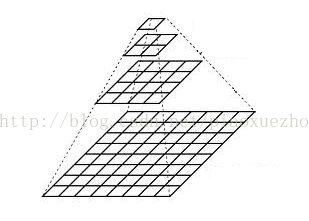
如上图所示,McCann99算法选取估计像素点是使用图像金字塔的方式逐层选取像素。
该算法利用图像金字塔建立多分辨率描述,自顶向下逐层迭代,提高增强效率。对输入图像的长宽有严格的限制。因为金字塔模型需要对输入图像进行下采样,金字塔上层低分辨率图像为下层高分辨率图像的1/2。
McCann99算法,此处简化描述为以下几步:
1. 将原图像变换到对数域S;
2. 初始化(计算图像金字塔层数;初始化常数图像矩阵R作为进行迭代运算的初始值);
3. 从顶层开始,到最后一层进行8邻域比较运算,运算规则与MccCann Retinex算法相同;
4. 第n层运算结束后对第n层的运算结果进行插值,变成原来的两倍,与n+1层大小相同;
5. 当最底层计算完毕得到的即最终增强后的图像。
下面是matlab函数实现:
function Retinex = retinex_mccann99(L, nIterations)

% RETINEX_McCANN99:
%         Computes the raw Retinex output from an intensity image, based on the
%         more recent model described in:
%         McCann, J., "Lessons Learned from Mondrians Applied to Real Images and
%         Color Gamuts", Proc. IS&T/SID Seventh Color Imaging Conference, pp. 1-8, 1999
%
% INPUT:  L           - logarithmic single-channel intensity image to be processed
%         nIterations - number of Retinex iterations
%
% OUTPUT: Retinex     - raw Retinex output
%
% NOTES:  - The input image is assumed to be logarithmic and in the range [0..1]
%         - To obtain the retinex "sensation" prediction, a look-up-table needs to
%         be applied to the raw retinex output
%         - For colour images, apply the algorithm individually for each channel


global OPE RRE Maximum
[nrows ncols] = size(L);                             % get size of the input image
nLayers = ComputeLayers(nrows, ncols);               % compute the number of pyramid layers
nrows = nrows/(2^nLayers);                           % size of image to process for layer 0
ncols = ncols/(2^nLayers);
if (nrows*ncols > 25000)                             % 阈值源程序为25,需要根据输入图像设置
  error('invalid image size.')                       % at first layer
end
Maximum = max(L(:));                                 % maximum color value in the image
OP = double(Maximum)*ones([nrows ncols]);                    % initialize Old Product
for layer = 0:nLayers
   RR = ImageDownResolution(L, 2^(nLayers-layer));   % reduce input to required layer size

   OPE = [zeros(nrows,1) OP zeros(nrows,1)];         % pad OP with additional columns
   OPE = [zeros(1,ncols+2); OPE; zeros(1,ncols+2)];  % and rows
   RRE = [RR(:,1) RR RR(:,end)];                     % pad RR with additional columns
   RRE = [RRE(1,:); RRE; RRE(end,:)];                % and rows

   for iter = 1:nIterations
     CompareWithNeighbor(-1, 0);                     % North
     CompareWithNeighbor(-1, 1);                     % North-East
     CompareWithNeighbor(0, 1);                      % East
     CompareWithNeighbor(1, 1);                      % South-East
     CompareWithNeighbor(1, 0);                      % South
     CompareWithNeighbor(1, -1);                     % South-West
     CompareWithNeighbor(0, -1);                     % West
     CompareWithNeighbor(-1, -1);                    % North-West
   end
   NP = OPE(2:(end-1), 2:(end-1));
   OP = NP(:, [fix(1:0.5:ncols) ncols]);             %%% these two lines are equivalent with
   OP = OP([fix(1:0.5:nrows) nrows], :);             %%% OP = imresize(NP, 2) if using Image
   nrows = 2*nrows; ncols = 2*ncols;                 % Processing Toolbox in MATLAB
end
Retinex = NP;

function CompareWithNeighbor(dif_row, dif_col)
global OPE RRE Maximum

% Ratio-Product operation
IP = OPE(2+dif_row:(end-1+dif_row), 2+dif_col:(end-1+dif_col)) + ...
     RRE(2:(end-1),2:(end-1)) - RRE(2+dif_row:(end-1+dif_row), 2+dif_col:(end-1+dif_col));

IP(IP > Maximum) = Maximum;                          % The Reset step

% ignore the results obtained in the rows or columns for which the neighbors are undefined
if (dif_col == -1) IP(:,1) = OPE(2:(end-1),2); end
if (dif_col == +1) IP(:,end) = OPE(2:(end-1),end-1); end
if (dif_row == -1) IP(1,:) = OPE(2, 2:(end-1)); end
if (dif_row == +1) IP(end,:) = OPE(end-1, 2:(end-1)); end
NP = (OPE(2:(end-1),2:(end-1)) + IP)/2;              % The Averaging operation
OPE(2:(end-1), 2:(end-1)) = NP;

function Layers = ComputeLayers(nrows, ncols)
power = 2^fix(log2(gcd(nrows, ncols)));              % start from the Greatest Common Divisor
while(power > 1 & ((rem(nrows, power) ~= 0) | (rem(ncols, power) ~= 0)))
   power = power/2;                                  % and find the greatest common divisor
end                                                  % that is a power of 2
Layers = log2(power);

function Result = ImageDownResolution(A, blocksize)
[rows, cols] = size(A);                              % the input matrix A is viewed as
result_rows = rows/blocksize;                        % a series of square blocks
result_cols = cols/blocksize;                        % of size = blocksize
Result = zeros([result_rows result_cols]);
for crt_row = 1:result_rows                          % then each pixel is computed as
   for crt_col = 1:result_cols                       % the average of each such block
      Result(crt_row, crt_col) = mean2(A(1+(crt_row-1)*blocksize:crt_row*blocksize, ...
                                       1+(crt_col-1)*blocksize:crt_col*blocksize));
   end
end
%% retinex99测试函数
clc,close all,clear all;
ImgOriginal=imread('../image/5.jpg');
[m,n,z] = size(ImgOriginal);
ImgOut = zeros(m,n,z);
nIterations=8;
for i = 1:z
ImChannel = log(double(ImgOriginal(:,:,i))+eps);
ImgOut(:,:,i)=retinex_mccann99(ImChannel,nIterations);
ImgOut(:,:,i)=exp(ImgOut(:,:,i));
a=min(min(ImgOut(:,:,i)));
b=max(max(ImgOut(:,:,i)));
ImgOut(:,:,i)=((ImgOut(:,:,i)-a)/(b-a))*255;
end
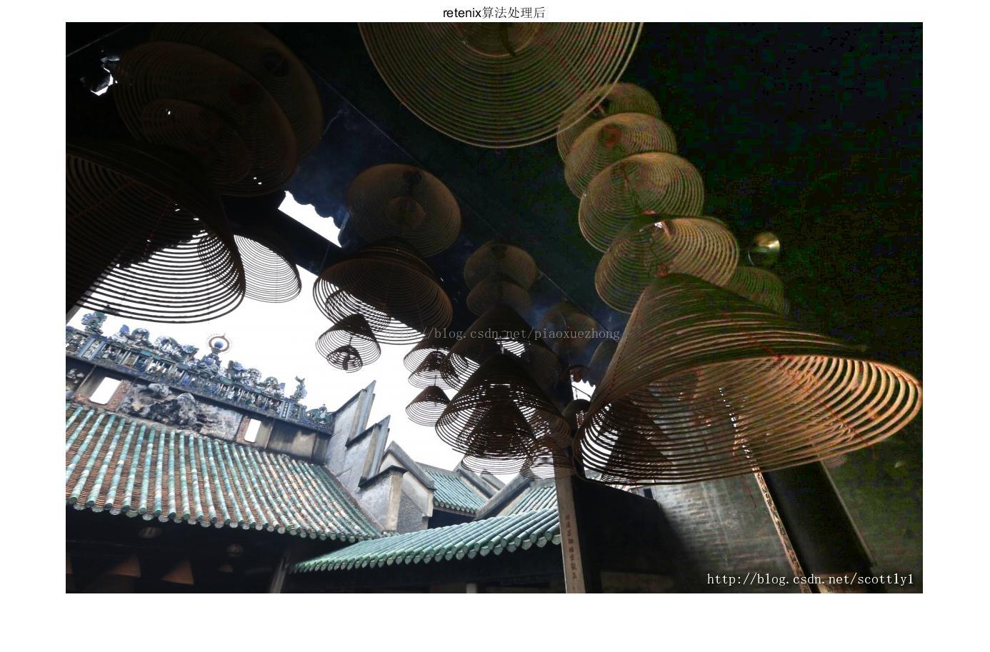
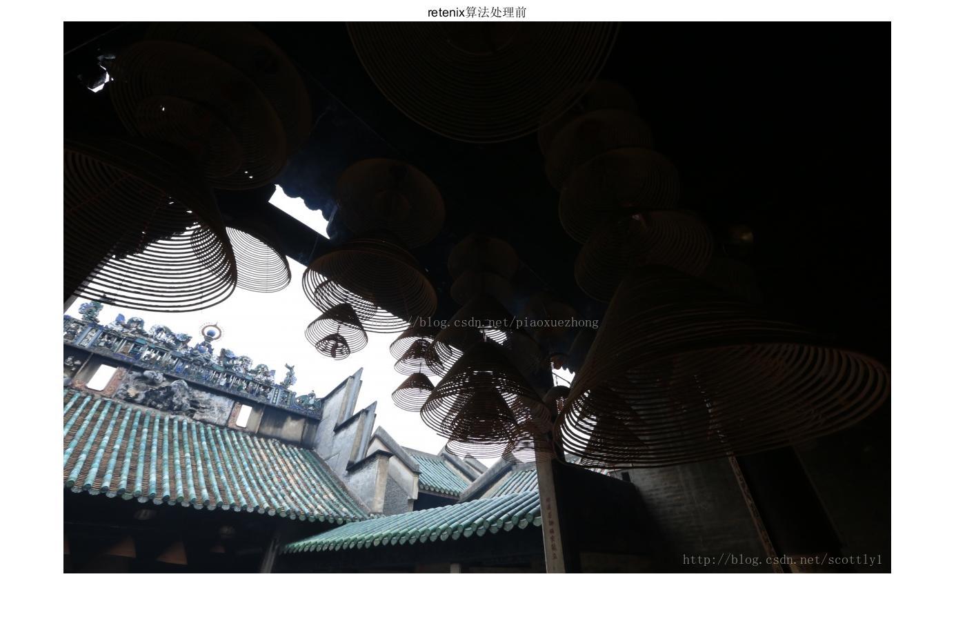
ImgOut=uint8(ImgOut);
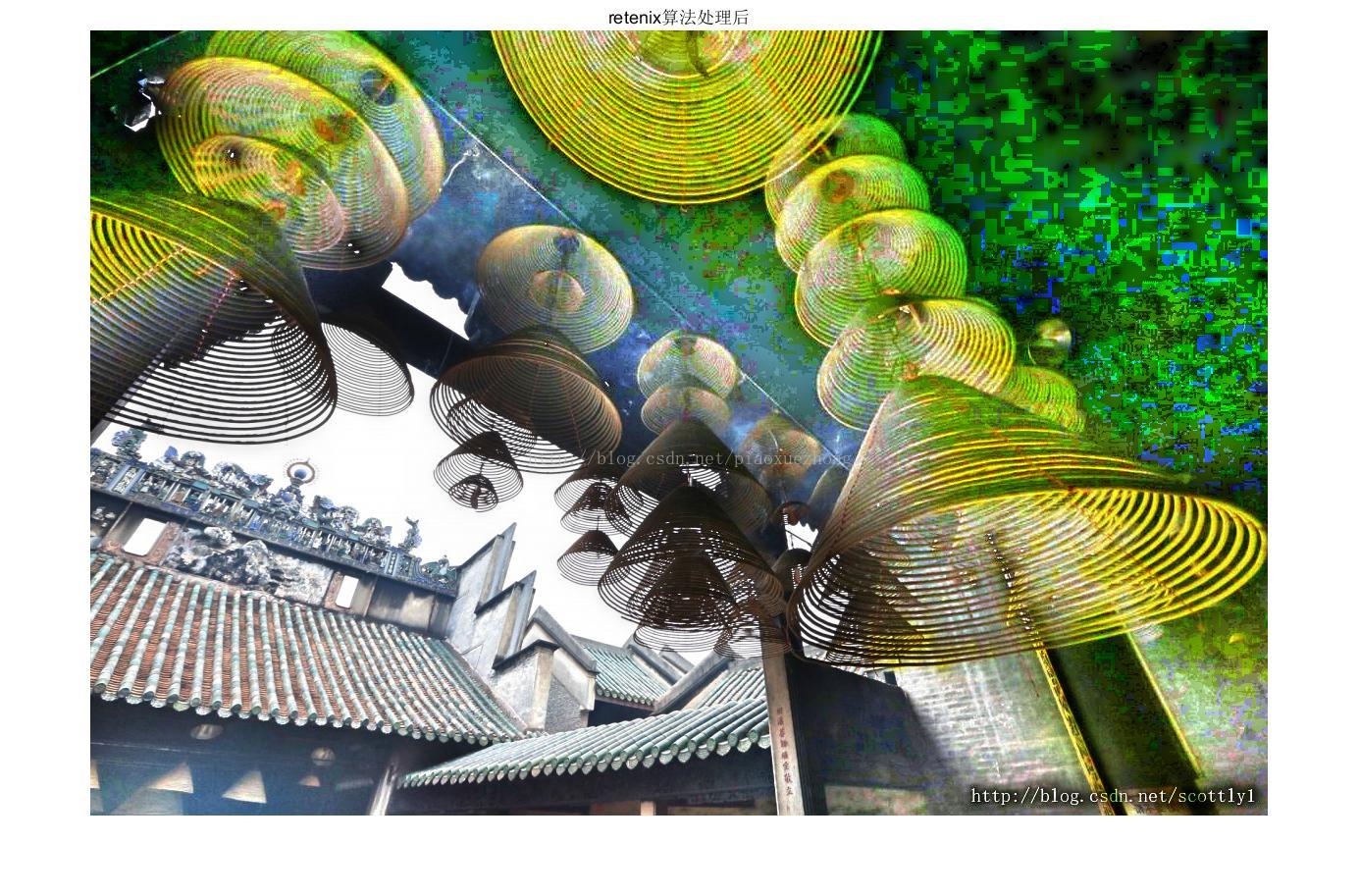
figure;
imshow(ImgOriginal); title('retenix算法处理前');
figure;
imshow(ImgOut); title('retenix算法处理后');
本来想继续写点Retinex邻域算法的东西,SSR,MSR,MSRCR等还是挺多的,后面单独一篇总结吧。
参考:
- http://blog.csdn.net/wangyaninglm/article/details/44651261
- http://www.cnblogs.com/sleepwalker/p/3676600.html?utm_source=tuicool&utm_medium=referral
- 图像去雾技术研究进展[J].中国图象图形学报
- http://blog.csdn.net/u010839382/article/details/41653343
- http://blog.csdn.net/u010839382/article/details/41694477


 2206
2206

 被折叠的 条评论
为什么被折叠?
被折叠的 条评论
为什么被折叠?
 到【灌水乐园】发言


