


今天给大家带来的是商品销售预测案例:
文件描述:
包括了销售数据数据集,测试集,店铺和商品以及商品种类等数据集。
sales_train.csv - the training set. Daily historical data from January 2013 to October 2015.
test.csv - the test set. You need to forecast the sales for these shops and products for November 2015.
sample_submission.csv - a sample submission file in the correct format.
items.csv - supplemental information about the items/products.
item_categories.csv  - supplemental information about the items categories.
shops.csv- supplemental information about the shops.
特征描述:
以上数据集的特征,有的是独有的,有的是公共的。
ID - an Id that represents a (Shop, Item) tuple within the test set
shop_id - unique identifier of a shop
item_id - unique identifier of a product
item_category_id - unique identifier of item category
item_cnt_day - number of products sold. You are predicting a monthly amount of this measure
item_price - current price of an item
date - date in format dd/mm/yyyy
date_block_num - a consecutive month number, used for convenience. January 2013 is 0, February 2013 is 1,..., October 2015 is 33
item_name - name of item
shop_name - name of shop
item_category_name - name of item category
导入数据:
数据集是来自俄罗斯,所有有些特征采用俄文书写。
import numpy as np
import pandas as pd
from sklearn import *
import nltk, datetime

train = pd.read_csv('D:/ML/Data/sales_train.csv/sales_train.csv')
test = pd.read_csv('D:/ML/Data/sales_train.csv/test.csv')
submission = pd.read_csv('D:/ML/Data/sales_train.csv/sample_submission.csv')
items = pd.read_csv('D:/ML/Data/sales_train.csv/items.csv')
item_cats = pd.read_csv('D:/ML/Data/sales_train.csv/item_categories.csv')
shops = pd.read_csv('D:/ML/Data/sales_train.csv/shops.csv')
print('train:', train.shape, 'test:', test.shape)
结果
train: (2935849, 6) test: (214200, 3)添加特征:
feature_cnt = 25
tfidf = feature_extraction.text.TfidfVectorizer(max_features=feature_cnt)
将原始文档的集合转换为TF-IDF功能的矩阵。
items['item_name_len'] = items['item_name'].map(len) #Lenth of Item Description
items['item_name_wc'] = items['item_name'].map(lambda x: len(str(x).split(' '))) #Item Description Word Count
txtFeatures = pd.DataFrame(tfidf.fit_transform(items['item_name']).toarray())
cols = txtFeatures.columns
for i in range(feature_cnt):
    items['item_name_tfidf_' + str(i)] = txtFeatures[cols[i]]
items.head()
运行结果:
item_name   item_id item_category_id    item_name_len   item_name_wc    item_name_tfidf_0   item_name_tfidf_1   item_name_tfidf_2   item_name_tfidf_3   item_name_tfidf_4   ... item_name_tfidf_15  item_name_tfidf_16  item_name_tfidf_17  item_name_tfidf_18  item_name_tfidf_19  item_name_tfidf_20  item_name_tfidf_21  item_name_tfidf_22  item_name_tfidf_23  item_name_tfidf_24
0   ! ВО ВЛАСТИ НАВАЖДЕНИЯ (ПЛАСТ.) D   0   40  41  14  0.0 0.0 0.0 0.0 0.0 ... 0.0 0.000000    0.0 0.0 0.0 0.0 0.0 0.0 0.0 0.000000
1   !ABBYY FineReader 12 Professional Edition Full...   1   76  68  9   0.0 0.0 0.0 0.0 0.0 ... 0.0 0.403761    0.0 0.0 0.0 0.0 0.0 0.0 0.0 0.483839
2   ***В ЛУЧАХ СЛАВЫ (UNV) D    2   40  45  26  0.0 0.0 0.0 0.0 0.0 ... 0.0 0.000000    0.0 0.0 0.0 0.0 0.0 0.0 0.0 0.000000
3   ***ГОЛУБАЯ ВОЛНА (Univ) D   3   40  47  26  0.0 0.0 0.0 0.0 0.0 ... 0.0 0.000000    0.0 0.0 0.0 0.0 0.0 0.0 0.0 0.000000
4   ***КОРОБКА (СТЕКЛО) D   4   40  43  25  0.0 0.0 0.0 0.0 0.0 ... 0.0 0.000000    0.0 0.0 0.0 0.0 0.0 0.0 0.0 0.000000
5 rows × 30 columns
在这里要重点介绍文本数据预处理:sklearn中CountVectorizer、TfidfTransformer和TfidfVectorizer
功能上来讲:TfidfVectorizer=CountVectorizer+TfidfTransformer
CountVectorizer是将文本数据的词频向量化
TfidfTransformer是将向量化之后的文本进行IF-IDF预处理
TfidfVectorizer可以一步完成二者的工作
接着进一步介绍TF-IDF:
TF-IDF(Term Frequency–Inverse Document Frequency)是一种用于资讯检索与文本挖掘的常用加权技术。TF-IDF是一种统计方法,用以评估一个字词对于一个文件集或一个语料库中的其中一份文件的重要程度。字词的重要性随着它在文件中出现的次数成正比增加,但同时会随着它在语料库中出现的频率成反比下降。TF-IDF加权的各种形式常被搜索引擎应用,作为文件与用户查询之间相关程度的度量或评级。
TF-IDF的主要思想是:如果某个词或短语在一篇文章中出现的频率TF高,并且在其他文章中很少出现,则认为此词或者短语具有很好的类别区分能力,适合用来分类。TF-IDF实际上是:TF * IDF。
词频(Term Frequency,TF)指的是某一个给定的词语在该文件中出现的频率。即词w在文档d中出现的次数count(w, d)和文档d中总词数size(d)的比值。
逆向文件频率(Inverse Document Frequency,IDF)是一个词语普遍重要性的度量。某一特定词语的IDF,可以由总文件数目除以包含该词语之文件的数目,再将得到的商取对数得到。即文档总数n与词w所出现文件数docs(w, D)比值的对数。
某一特定文件内的高词语频率,以及该词语在整个文件集合中的低文件频率,可以产生出高权重的TF-IDF。因此,TF-IDF倾向于过滤掉常见的词语,保留重要的词语。
#Text Features
feature_cnt = 25
tfidf = feature_extraction.text.TfidfVectorizer(max_features=feature_cnt)
item_cats['item_category_name_len'] = item_cats['item_category_name'].map(len)  #Lenth of Item Category Description
item_cats['item_category_name_wc'] = item_cats['item_category_name'].map(lambda x: len(str(x).split(' '))) #Item Category Description Word Count
txtFeatures = pd.DataFrame(tfidf.fit_transform(item_cats['item_category_name']).toarray())
cols = txtFeatures.columns
for i in range(feature_cnt):
    item_cats['item_category_name_tfidf_' + str(i)] = txtFeatures[cols[i]]
item_cats.head()
item_category_name item_category_id item_category_name_len item_category_name_wc item_category_name_tfidf_0 item_category_name_tfidf_1 item_category_name_tfidf_2 item_category_name_tfidf_3 item_category_name_tfidf_4 item_category_name_tfidf_5 ... item_category_name_tfidf_15 item_category_name_tfidf_16 item_category_name_tfidf_17 item_category_name_tfidf_18 item_category_name_tfidf_19 item_category_name_tfidf_20 item_category_name_tfidf_21 item_category_name_tfidf_22 item_category_name_tfidf_23 item_category_name_tfidf_24
0 PC - Гарнитуры/Наушники 0 23 3 0.0 0.0 0.0 1.0 0.000000 0.000000 ... 0.0 0.0 0.0 0.0 0.0 0.0 0.0 0.0 0.0 0.0
1 Аксессуары - PS2 1 16 3 0.0 0.0 0.0 0.0 0.780837 0.000000 ... 0.0 0.0 0.0 0.0 0.0 0.0 0.0 0.0 0.0 0.0
2 Аксессуары - PS3 2 16 3 0.0 0.0 0.0 0.0 0.000000 0.780837 ... 0.0 0.0 0.0 0.0 0.0 0.0 0.0 0.0 0.0 0.0
3 Аксессуары - PS4 3 16 3 0.0 0.0 0.0 0.0 0.000000 0.000000 ... 0.0 0.0 0.0 0.0 0.0 0.0 0.0 0.0 0.0 0.0
4 Аксессуары - PSP 4 16 3 0.0 0.0 0.0 0.0 0.000000 0.000000 ... 0.0 0.0 0.0 0.0 0.0 0.0 0.0 0.0 0.0 0.0
5 rows × 29 columns#Text Features
feature_cnt = 25
tfidf = feature_extraction.text.TfidfVectorizer(max_features=feature_cnt)
shops['shop_name_len'] = shops['shop_name'].map(len) #Lenth of Shop Name
shops['shop_name_wc'] = shops['shop_name'].map(lambda x: len(str(x).split(' '))) #Shop Name Word Count
txtFeatures = pd.DataFrame(tfidf.fit_transform(shops['shop_name']).toarray())
cols = txtFeatures.columns
for i in range(feature_cnt):
shops['shop_name_tfidf_' + str(i)] = txtFeatures[cols[i]]
shops.head() shop_name shop_id shop_name_len shop_name_wc shop_name_tfidf_0 shop_name_tfidf_1 shop_name_tfidf_2 shop_name_tfidf_3 shop_name_tfidf_4 shop_name_tfidf_5 ... shop_name_tfidf_15 shop_name_tfidf_16 shop_name_tfidf_17 shop_name_tfidf_18 shop_name_tfidf_19 shop_name_tfidf_20 shop_name_tfidf_21 shop_name_tfidf_22 shop_name_tfidf_23 shop_name_tfidf_24
0 !Якутск Орджоникидзе, 56 фран 0 29 4 0.0 0.0 0.0 0.0 0.0 0.0 ... 0.0 0.0 0.0 0.0 0.0 0.0 0.000000 0.0 0.000000 1.000000
1 !Якутск ТЦ "Центральный" фран 1 29 4 0.0 0.0 0.0 0.0 0.0 0.0 ... 0.0 0.0 0.0 0.0 0.0 0.0 0.322815 0.0 0.689588 0.648274
2 Адыгея ТЦ "Мега" 2 16 3 0.0 0.0 0.0 0.0 0.0 0.0 ... 0.0 0.0 0.0 0.0 0.0 0.0 0.498580 0.0 0.000000 0.000000
3 Балашиха ТРК "Октябрь-Киномир" 3 30 3 0.0 0.0 0.0 0.0 0.0 0.0 ... 0.0 0.0 0.0 0.0 1.0 0.0 0.000000 0.0 0.000000 0.000000
4 Волжский ТЦ "Волга Молл" 4 24 4 0.0 0.0 0.0 0.0 0.0 0.0 ... 0.0 0.0 0.0 0.0 0.0 0.0 0.423972 0.0 0.000000 0.000000
5 rows × 29 columnstrain['date'] = pd.to_datetime(train['date'], format='%d.%m.%Y')
train['month'] = train['date'].dt.month
train['year'] = train['date'].dt.year
train = train.drop(['date','item_price'], axis=1)
train = train.groupby([c for c in train.columns if c not in ['item_cnt_day']], as_index=False)[['item_cnt_day']].sum()
train = train.rename(columns={'item_cnt_day':'item_cnt_month'})
#Monthly Mean
shop_item_monthly_mean = train[['shop_id','item_id','item_cnt_month']].groupby(['shop_id','item_id'], as_index=False)[['item_cnt_month']].mean()
shop_item_monthly_mean = shop_item_monthly_mean.rename(columns={'item_cnt_month':'item_cnt_month_mean'})
#Add Mean Feature
train = pd.merge(train, shop_item_monthly_mean, how='left', on=['shop_id','item_id'])
#Last Month (Oct 2015)
shop_item_prev_month = train[train['date_block_num']==33][['shop_id','item_id','item_cnt_month']]
shop_item_prev_month = shop_item_prev_month.rename(columns={'item_cnt_month':'item_cnt_prev_month'})
shop_item_prev_month.head()
#Add Previous Month Feature
train = pd.merge(train, shop_item_prev_month, how='left', on=['shop_id','item_id']).fillna(0.)
#Items features
train = pd.merge(train, items, how='left', on='item_id')
#Item Category features
train = pd.merge(train, item_cats, how='left', on='item_category_id')
#Shops features
train = pd.merge(train, shops, how='left', on='shop_id')
train.head() date_block_num shop_id item_id month year item_cnt_month item_cnt_month_mean item_cnt_prev_month item_name item_category_id ... shop_name_tfidf_15 shop_name_tfidf_16 shop_name_tfidf_17 shop_name_tfidf_18 shop_name_tfidf_19 shop_name_tfidf_20 shop_name_tfidf_21 shop_name_tfidf_22 shop_name_tfidf_23 shop_name_tfidf_24
0 0 0 32 1 2013 6.0 8.0 0.0 1+1 40 ... 0.0 0.0 0.0 0.0 0.0 0.0 0.0 0.0 0.0 1.0
1 0 0 33 1 2013 3.0 3.0 0.0 1+1 (BD) 37 ... 0.0 0.0 0.0 0.0 0.0 0.0 0.0 0.0 0.0 1.0
2 0 0 35 1 2013 1.0 7.5 0.0 10 ЛЕТ СПУСТЯ 40 ... 0.0 0.0 0.0 0.0 0.0 0.0 0.0 0.0 0.0 1.0
3 0 0 43 1 2013 1.0 1.0 0.0 100 МИЛЛИОНОВ ЕВРО 40 ... 0.0 0.0 0.0 0.0 0.0 0.0 0.0 0.0 0.0 1.0
4 0 0 51 1 2013 2.0 2.5 0.0 100 лучших произведений классики (mp3-CD) (Dig... 57 ... 0.0 0.0 0.0 0.0 0.0 0.0 0.0 0.0 0.0 1.0
5 rows × 93 columnstest['month'] = 11
test['year'] = 2015
test['date_block_num'] = 34
#Add Mean Feature
test = pd.merge(test, shop_item_monthly_mean, how='left', on=['shop_id','item_id']).fillna(0.)
#Add Previous Month Feature
test = pd.merge(test, shop_item_prev_month, how='left', on=['shop_id','item_id']).fillna(0.)
#Items features
test = pd.merge(test, items, how='left', on='item_id')
#Item Category features
test = pd.merge(test, item_cats, how='left', on='item_category_id')
#Shops features
test = pd.merge(test, shops, how='left', on='shop_id')
test['item_cnt_month'] = 0.
test.head() ID shop_id item_id month year date_block_num item_cnt_month_mean item_cnt_prev_month item_name item_category_id ... shop_name_tfidf_16 shop_name_tfidf_17 shop_name_tfidf_18 shop_name_tfidf_19 shop_name_tfidf_20 shop_name_tfidf_21 shop_name_tfidf_22 shop_name_tfidf_23 shop_name_tfidf_24 item_cnt_month
0 0 5 5037 11 2015 34 1.444444 0.0 NHL 15 [PS3, русские субтитры] 19 ... 0.0 0.0 0.0 0.0 1.0 0.0 0.0 0.0 0.0 0.0
1 1 5 5320 11 2015 34 0.000000 0.0 ONE DIRECTION Made In The A.M. 55 ... 0.0 0.0 0.0 0.0 1.0 0.0 0.0 0.0 0.0 0.0
2 2 5 5233 11 2015 34 2.000000 1.0 Need for Speed Rivals (Essentials) [PS3, русск... 19 ... 0.0 0.0 0.0 0.0 1.0 0.0 0.0 0.0 0.0 0.0
3 3 5 5232 11 2015 34 1.000000 0.0 Need for Speed Rivals (Classics) [Xbox 360, ру... 23 ... 0.0 0.0 0.0 0.0 1.0 0.0 0.0 0.0 0.0 0.0
4 4 5 5268 11 2015 34 0.000000 0.0 Need for Speed [PS4, русская версия] 20 ... 0.0 0.0 0.0 0.0 1.0 0.0 0.0 0.0 0.0 0.0
5 rows × 94 columns可视化结果:
from PIL import Image, ImageDraw, ImageFilter
import matplotlib.pyplot as plt
import seaborn as sns
%matplotlib inline

df_all = pd.concat((train, test), axis=0, ignore_index=True)
stores_hm = df_all.pivot_table(index='shop_id', columns='item_category_id', values='item_cnt_month', aggfunc='count', fill_value=0)
fig, ax = plt.subplots(figsize=(10,10))
_ = sns.heatmap(stores_hm, ax=ax, cbar=False)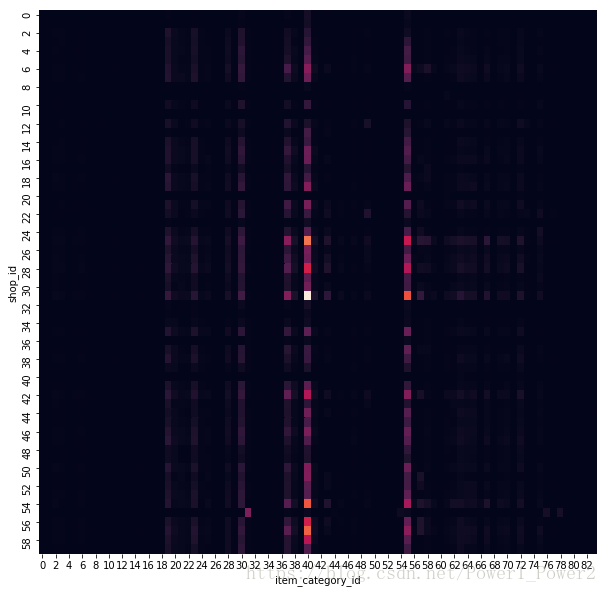
stores_hm = test.pivot_table(index='shop_id', columns='item_category_id', values='item_cnt_month', aggfunc='count', fill_value=0)
fig, ax = plt.subplots(figsize=(10,10))
_ = sns.heatmap(stores_hm, ax=ax, cbar=False)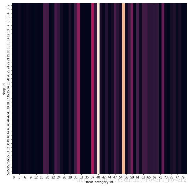
for c in ['shop_name','item_name','item_category_name']:
    lbl = preprocessing.LabelEncoder()
    lbl.fit(list(train[c].unique())+list(test[c].unique()))
    train[c] = lbl.transform(train[c].astype(str))
    test[c] = lbl.transform(test[c].astype(str))
    print(c)
shop_name
item_name
item_category_name模型训练:
col = [c for c in train.columns if c not in ['item_cnt_month']]
#Validation Hold Out Month
x1 = train[train['date_block_num']<33]
y1 = np.log1p(x1['item_cnt_month'].clip(0.,20.))
x1 = x1[col]
x2 = train[train['date_block_num']==33]
y2 = np.log1p(x2['item_cnt_month'].clip(0.,20.))
x2 = x2[col]

reg = ensemble.ExtraTreesRegressor(n_estimators=25, n_jobs=-1, max_depth=15, random_state=18)
reg.fit(x1,y1)
print('RMSE:', np.sqrt(metrics.mean_squared_error(y2.clip(0.,20.),reg.predict(x2).clip(0.,20.))))
#full train
reg.fit(train[col],train['item_cnt_month'].clip(0.,20.))
test['item_cnt_month'] = reg.predict(test[col]).clip(0.,20.)
test[['ID','item_cnt_month']].to_csv('submission.csv', index=False)RMSE: 0.27595668657276884import xgboost as xgb
import lightgbm as lgb
from catboost import CatBoostRegressor
from multiprocessing import *
#XGBoost
def xgb_rmse(preds, y):
y = y.get_label()
score = np.sqrt(metrics.mean_squared_error(y.clip(0.,20.), preds.clip(0.,20.)))
return 'RMSE', score
params = {'eta': 0.2, 'max_depth': 4, 'objective': 'reg:linear', 'eval_metric': 'rmse', 'seed': 18, 'silent': True}
#watchlist = [(xgb.DMatrix(x1, y1), 'train'), (xgb.DMatrix(x2, y2), 'valid')]
#xgb_model = xgb.train(params, xgb.DMatrix(x1, y1), 100, watchlist, verbose_eval=10, feval=xgb_rmse, maximize=False, early_stopping_rounds=20)
#test['item_cnt_month'] = xgb_model.predict(xgb.DMatrix(test[col]), ntree_limit=xgb_model.best_ntree_limit)
#test[['ID','item_cnt_month']].to_csv('xgb_submission.csv', index=False)
#LightGBM
def lgb_rmse(preds, y):
y = np.array(list(y.get_label()))
score = np.sqrt(metrics.mean_squared_error(y.clip(0.,20.), preds.clip(0.,20.)))
return 'RMSE', score, False
params = {'learning_rate': 0.2, 'max_depth': 7, 'boosting': 'gbdt', 'objective': 'regression', 'metric': 'mse', 'is_training_metric': False, 'seed': 18}
#lgb_model = lgb.train(params, lgb.Dataset(x1, label=y1), 100, lgb.Dataset(x2, label=y2), feval=lgb_rmse, verbose_eval=10, early_stopping_rounds=20)
#test['item_cnt_month'] = lgb_model.predict(test[col], num_iteration=lgb_model.best_iteration)
#test[['ID','item_cnt_month']].to_csv('lgb_submission.csv', index=False)
#CatBoost
cb_model = CatBoostRegressor(iterations=100, learning_rate=0.2, depth=7, loss_function='RMSE', eval_metric='RMSE', random_seed=18, od_type='Iter', od_wait=20)
cb_model.fit(x1, y1, eval_set=(x2, y2), use_best_model=True, verbose=False)
print('RMSE:', np.sqrt(metrics.mean_squared_error(y2.clip(0.,20.), cb_model.predict(x2).clip(0.,20.))))
test['item_cnt_month'] += cb_model.predict(test[col])
test['item_cnt_month'] /= 2
test[['ID','item_cnt_month']].to_csv('cb_blend_submission.csv', index=False)RMSE: 0.2735090078825704


 6654
6654


 被折叠的 条评论
为什么被折叠?
被折叠的 条评论
为什么被折叠?
 到【灌水乐园】发言


