GEE必须会教程——Savitzky-Golay（S-G）滤波器在MODIS影像时间序列数据的应用

今天比较懒，不想多写文字啦，还记得昨天分享的S-G滤波器，大家有没有去试试。今天布置个任务，同样以昨天的研究区域为例，试试看MODIS时间序列数据如何实现平滑！

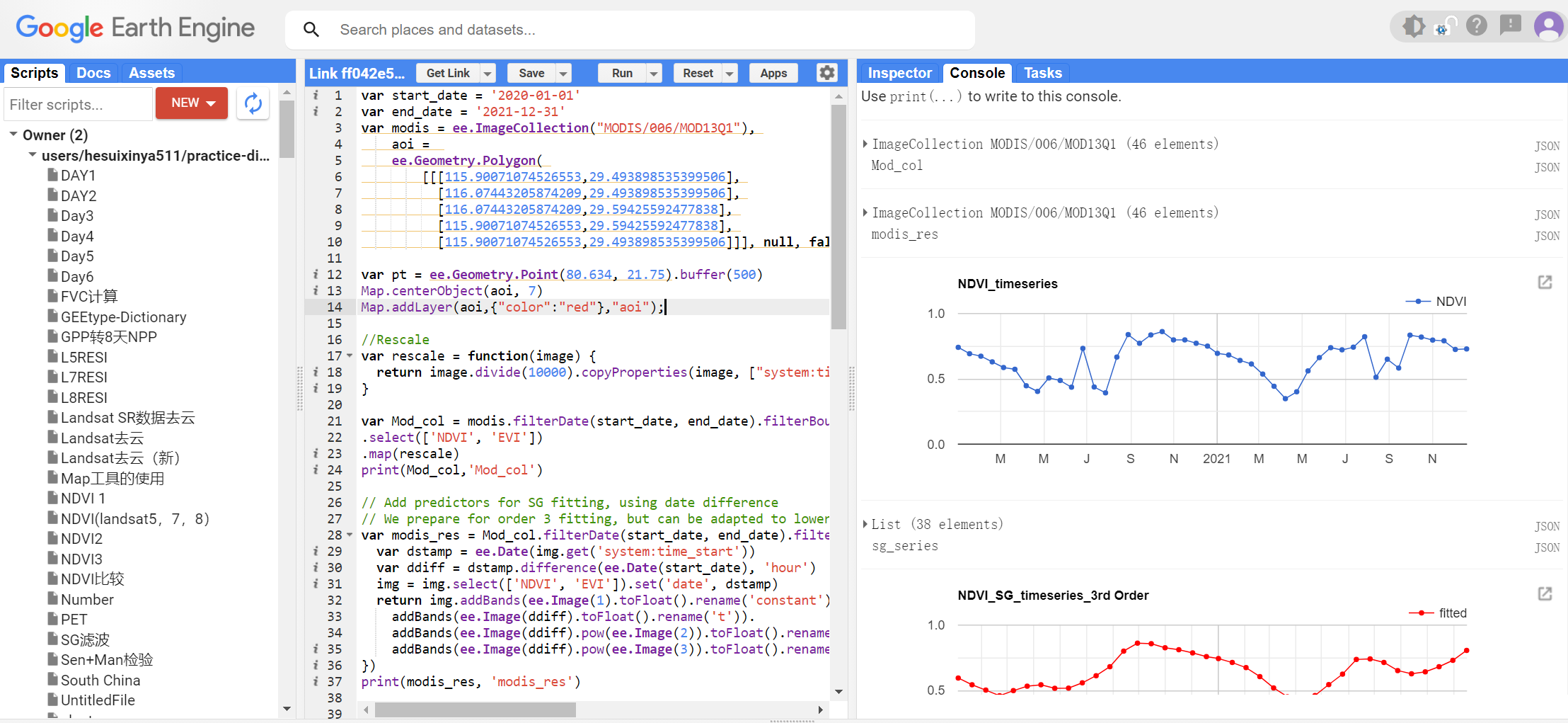
话不多说，今天直接上代码吧

var start_date = '2020-01-01'
var end_date = '2021-12-31'
var modis = ee.ImageCollection("MODIS/006/MOD13Q1"),
    aoi = 
    ee.Geometry.Polygon(
        [[[115.90071074526553,29.493898535399506],
          [116.07443205874209,29.493898535399506],
          [116.07443205874209,29.59425592477838],
          [115.90071074526553,29.59425592477838],
          [115.90071074526553,29.493898535399506]]], null, false);

var pt = ee.Geometry.Point(80.634, 21.75).buffer(500)
Map.centerObject(aoi, 7)
Map.addLayer(aoi,{"color":"red"},"aoi");

//Rescale
var rescale = function(image) {
  return image.divide(10000).copyProperties(image, ["system:time_start", "system:time_end"])
}

var Mod_col = modis.filterDate(start_date, end_date).filterBounds(pt)
.select(['NDVI', 'EVI'])
.map(rescale)
print(Mod_col,'Mod_col')

// Add predictors for SG fitting, using date difference
// We prepare for order 3 fitting, but can be adapted to lower order fitting later on
var modis_res = Mod_col.filterDate(start_date, end_date).filterBounds(aoi).map(function(img) {
  var dstamp = ee.Date(img.get('system:time_start'))
  var ddiff = dstamp.difference(ee.Date(start_date), 'hour')
  img = img.select(['NDVI', 'EVI']).set('date', dstamp)
  return img.addBands(ee.Image(1).toFloat().rename('constant')).
    addBands(ee.Image(ddiff).toFloat().rename('t')).
    addBands(ee.Image(ddiff).pow(ee.Image(2)).toFloat().rename('t2')).
    addBands(ee.Image(ddiff).pow(ee.Image(3)).toFloat().rename('t3'))
})
print(modis_res, 'modis_res')


print(Chart.image.series(modis_res.select('NDVI'), pt, ee.Reducer.mean(), 500)//.select('NDVI')
    //.setSeriesNames(['fitted'])
    .setOptions({
      title: 'NDVI_timeseries',
      lineWidth: 1,
      pointSize: 3,
}));

// Step 2: Set up Savitzky-Golay smoothing
var window_size = 9
var half_window = (window_size - 1)/2

// Define the axes of variation in the collection array.
var imageAxis = 0;
var bandAxis = 1;

// Set polynomial order
var order = 3
var coeffFlattener = [['constant', 'x', 'x2', 'x3']]
var indepSelectors = ['constant', 't', 't2', 't3']

// Convert the collection to an array.
var array = modis_res.toArray();

// Solve 
function getLocalFit(i) {
  // Get a slice corresponding to the window_size of the SG smoother
  var subarray = array.arraySlice(imageAxis, ee.Number(i).int(), ee.Number(i).add(window_size).int())
  var predictors = subarray.arraySlice(bandAxis, 2, 2 + order + 1)
  var response = subarray.arraySlice(bandAxis, 0, 1); // NDVI
  var coeff = predictors.matrixSolve(response)

  coeff = coeff.arrayProject([0]).arrayFlatten(coeffFlattener)
  return coeff  
}

// For the remainder, use modis_res as a list of images
modis_res = modis_res.toList(modis_res.size())

var runLength = ee.List.sequence(0, modis_res.size().subtract(window_size))

// Run the SG filter over the series, and get the smoothed image 
var sg_series = runLength.map(function(i) {
  var ref = ee.Image(modis_res.get(ee.Number(i).add(half_window)))
  return getLocalFit(i).multiply(ref.select(indepSelectors)).reduce(ee.Reducer.sum()).copyProperties(ref,['date','system:time_start'])
})
print(sg_series, 'sg_series')

print(Chart.image.series(sg_series, pt, ee.Reducer.mean(), 500)
    .setSeriesNames(['fitted'])
    .setOptions({
      title: 'NDVI_SG_timeseries_3rd Order',
      lineWidth: 1,
      pointSize: 3,
      colors:["#FF0000"]
}));

看一波结果：

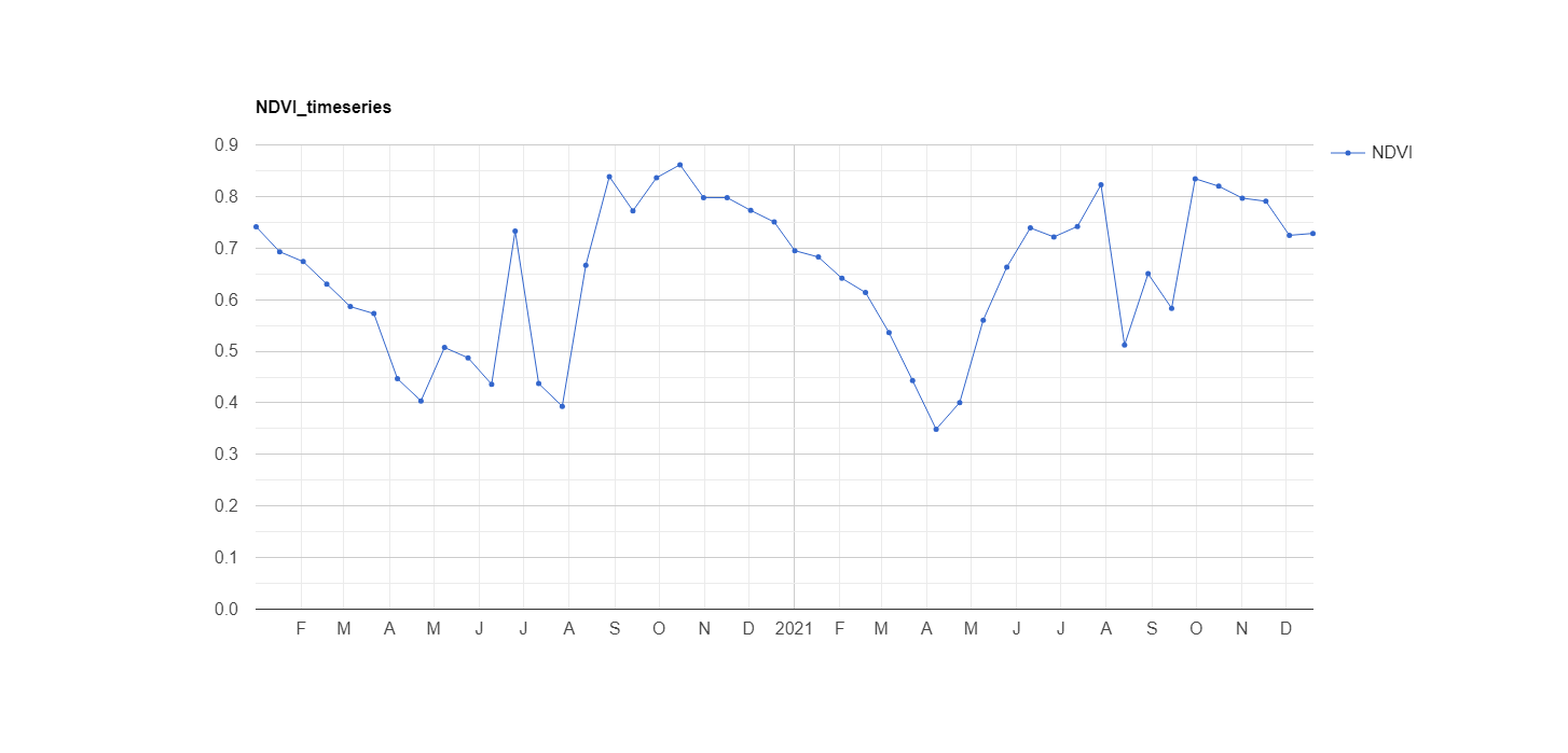
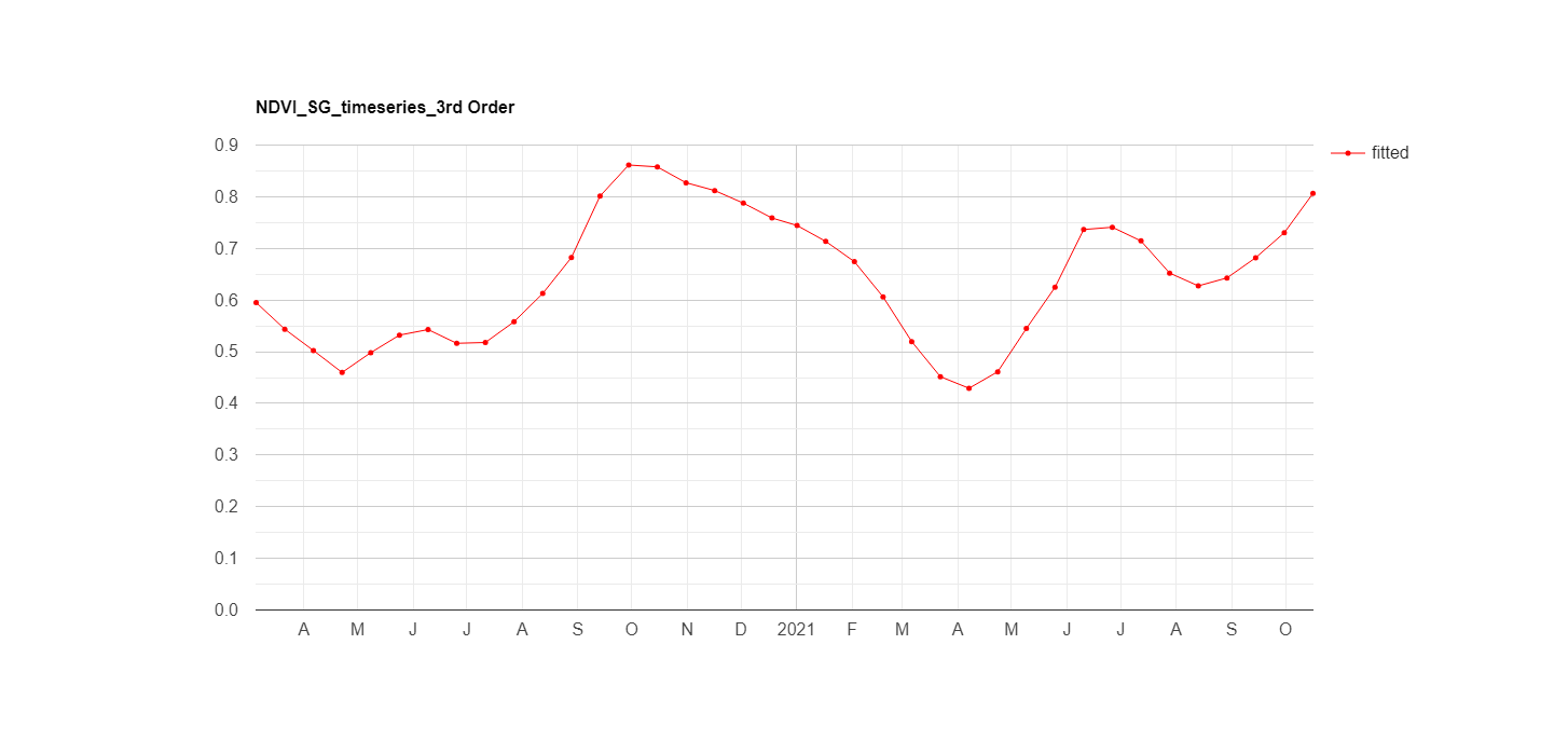
结果还比较赏心悦目，好啦好啦，开启元气满满新一天！！

好了，今天的分享到这里就结束了，更多内容欢迎持续关注小编的公众号“梧桐GIS”，我是禾穗，咱们下期再会啦！！