机器学习之概率密度估计

写在前面的话： 本文简述概率密度估计的方法以及代码实现，其中包括 极大似然估计 和 非参数方法， 非参数方法包括 parzen窗 和 knn(k近邻)算法。注意，重点不是推导过程，而是最最最基本的实现方法！代码是用python，老师给的是.mat文件，本意是matlab，奈何我没好好学。代码也不够简单，欢迎批评。都是手动实现，knn用集成库也实现了一下，确实简单粗暴。
在文末会放入几篇个人认为比较容易理解的链接。

基本问题： 已知一定数目的样本（类别已知），对未知样本分类，转化为数学语言就是——已知?(?_? )和?(?|?_?)对未知样本分类

• 首先根据样本估计 $p(x|w_i)$ 和 $p(w_i)$，记 $\hat{p}(x|w_i)$ 和 $\hat{p}(x|w_i)$
• 然后用估计的概率密度设计贝叶斯分类器

重要前提

• 训练样本的分布能代表样本的真实分布，样本满足独立同分布条件–independent and identically distributed (i.i.d条件)
• 有充分的训练样本

关键就是求 $p(x|w_i)$ ！

一. 参数估计 (parametric methods)

已知概率密度函数 $p(x|w_i)$ 的形式，只是其中几个参数未知，目标是根据样本估计这些参数的值。

最大似然估计(Maximum Likelihood Estimation)

$$l(\theta )=p(x|\theta )=\prod _{i=1}^{N}p(x_i|\theta )$$

我来大白话解释一下，样本集 x已知，而参数 ? 未知, ?(?)反映的是不同 ? 取值下，取得当前样本的可能性。取得值最大的那个 ? 就是我们需要的。为便于计算，令

$$H(\theta )=\prod _{i=1}^{N}lnp(x_i|\theta )$$

求偏导过程略过，直接得出结论

• 单变正态分布
  $$\hat{u}={\hat{\theta }}_1=\frac{1}{N}\sum _{i=1}^N{x}_i$$

$${\hat{\sigma }}^2={\hat{\theta }}_2=\frac{1}{N}\sum _{i=1}^N(x_i-\hat{u}{)}^2$$

• 多元正态分布
  $$\vec{\hat{u}}={\hat{\theta }}_1=\frac{1}{N}\sum _{i=1}^N\overrightarrow{x_i}$$

$$\vec{\hat{\sigma }}\frac{1}{N}\sum _{i=1}^N(\overrightarrow{x_i}-\vec{\hat{u}})(\overrightarrow{x_i}-\vec{\hat{u}}{)}^T$$

---

例题

“data_lab_threeD.mat”文件中包括三类样本，样本总数量为999，在该数据中每一列为一个样本，前三行为每一个样本的特征，第四行为该样本的类别信息，如下所示：

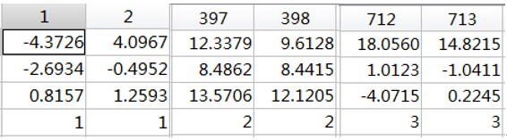
考虑不同维度下的高斯概率密度模型。
（1） 编写程序，对“data_lab_threeD.mat”中类别为“1”的数据，分别计算每个特征xi下的最大似然估计μ ̂和σ ̂^2。
（2）编写程序，对“data_lab_threeD.mat”中类别为“1”的数据，计算特征组合x下的最大似然估计μ ̂和Σ ̂。

import scipy.io as si
import numpy as np
import pandas as pd

def get_datas(path):
    data = si.loadmat(path)
    datas = data['data_lab_threeD']
    datas = pd.DataFrame(datas.T, columns=['x1','x2','x3', 'class'])
    Xs = [[x1,x2,x3] for x1,x2,x3 in zip(datas['x1'], datas['x2'], datas['x3'])]
    return Xs, datas

def calculate_mean(li):
    count = 0
    u = np.sum(li) / len(li)
    for i in li:
        count += (i-u)**2
    count = count/len(li)
    
    return u, count

def per_feature(Xs, datas):
    grouped = datas.groupby('class')
    class1 = grouped.get_group(1)

    x1 = list(class1.x1)
    x2 = list(class1.x2)
    x3 = list(class1.x3)
    
    u1, theta1 = calculate_mean(x1)
    u1, theta2 = calculate_mean(x2)
    u1, theta3 = calculate_mean(x3)
    
    u = np.matrix([u1, u2, u3]).T
    for i in range(len(Xs)):
        sigma = np.sum((np.matrix(Xs[i]).T - u) * (np.matrix(Xs[i]).T - u).T) / len(class1)

    for i,j,k in zip([u1,u2,u3],[theta1, theta2, theta3],[1,2,3]):
        print("the x{}'s maximum likelihood estimation is {:.4f} and {:.4f}".format(k,i,j))
        
    print("the matrix x's maximum likelihood estimation is \n{} and {}".format(u, sigma))

if __name__ == '__main__':   
    
    path = './data_lab_threeD.mat'
    X, datas = get_datas(path)
    per_feature(X, datas)

Outcome:

the x1's maximum likelihood estimation is 0.9270 and 3.7744
the x2's maximum likelihood estimation is 1.0327 and 3.9120
the x3's maximum likelihood estimation is 0.9270 and 3.3836
the matrix x's maximum likelihood estimation is 
[[0.92699263]
 [1.03271502]
 [0.92699263]] and 1.1733159529664747

---

二. 非参数估计(parametric methodsnonparametric estimation)

• 不对 $p(x|w_i)$ 的形式进行假设，直接用样本估计 $p(x|w_i)$
• 只能得到数值解，无法得到封闭解

基本条件：

1. 要求样本数目足够大
2. 计算量和存储量大
3. 适用于任何概率密度的估计

先写一个最 基本的公式：
$$p(x)=\frac{k_x}{NV}$$

大白话到了！！！ 同体积比较个数，同个数比较体积。( 体积属于维度概念，不限于三维 )，parzen是后者，knn是前者。

1. Parzen 窗法

若特征 $x$ 是 $d$ 维，每维的棱长为 $h$ ，则小舱的体积 $V=h^d$
$N$ 个观测样本 { x 1 , x 2 , … , x N } \{x_1,x_2,…,x_N\} {x1​,x2​,…,xN​}
对于每个 $x$，考察样本 $x_i$ 是否落入以 $x$ 为中心，$h$ 为棱长的小舱内。

2. $k_N$ 近邻估计

样本密度高的地方，小舱体积小
样本密度低的地方，小舱体积大

看了那么多，其实就一句话： 首先明白，k是自己定义的参数——最短距离的个数。求测试集与每个训练集的距离 ( 多用欧式距离 )，升序排序取前k个，这k个里哪个类别最多就判别为哪个类就ok了！

---

例题

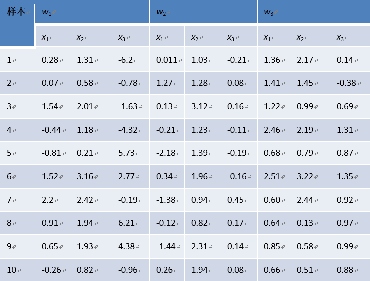
1.考虑对于表格中的数据进行parzen窗估计和设计分类器，窗函数为一个球形的高斯函数。
编写程序，使用parzen窗估计方法对一个任意的样本点x进行分类。对分类器的训练使用表格中的三维数据，分类样本点为
(0.5,1.0,0.0)T， (0.31, 1.51, -0.50) T，(-0.3, 0.44, -0.1)
(a) h=1
(b) h=0.1

2.考虑对于表格中的数据进行k_N 近邻概率密度估计和设计分类器。
编写程序，使用k_N 近邻估计方法对一个任意的样本点x进行分类。对分类器的训练使用表格中的三维数据，分类样本点为
(0.5,1.0,0.0)T， (0.31, 1.51, -0.50) T，(-0.3, 0.44, -0.1)。。
（a）k=1
（b）k=3
（c）k=5

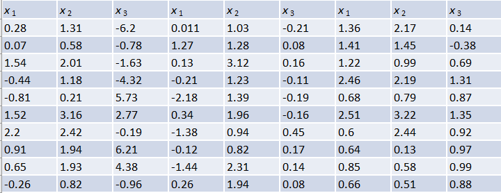
由于数据量小，这个表格我先放到了excel里，便于编程

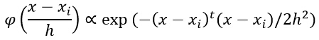
第一题数据格式及公式如下图（公式忽略了除以体积）

import numpy as np
import pandas as pd

def parzen(Xs, x, h):
    
    px = 0 
    vn = 4 * np.pi * h**3 /3
    for i in range(len(Xs)):
        px += np.exp(-(x - (np.matrix(Xs[i]).T)).T * (x - (np.matrix(Xs[i]).T)) / (2 * h**2)) / vn
    
    px = px / 3
    return px

def get_best_class(datas, x,h):
    
    Xs1 = [[x1,x2,x3] for x1,x2,x3 in zip(datas['x11'], datas['x12'], datas['x13'])]
    Xs2 = [[x1,x2,x3] for x1,x2,x3 in zip(datas['x21'], datas['x22'], datas['x23'])]
    Xs3 = [[x1,x2,x3] for x1,x2,x3 in zip(datas['x31'], datas['x32'], datas['x33'])]
    
    p11 = parzen(Xs1, x, h)
    p12 = parzen(Xs2, x, h)
    p13 = parzen(Xs3, x, h)
    
    maximum = max(p11, p12, p13)
    print("when h = {}\t".format(h))
    if p11 == maximum:
        print("the num {} belongs to 'w1'".format(x.T))
    elif p12 == maximum:
        print("the num {} belongs to 'w2'".format(x.T))
    else:
        print("the num {} belongs to 'w3'".format(x.T))

df = pd.read_excel('./params.xlsx', encoding='utf-8')
df.columns = ['x11', 'x12', 'x13', 'x21', 'x22', 'x23', 'x31', 'x32', 'x33']

x1 = np.matrix([0.5,1.0,0.0]).T
x2 = np.matrix([0.31, 1.51, -0.50]).T
x3 = np.matrix([-0.3, 0.44, -0.1]).T

get_best_class(df, x1, 1)
get_best_class(df, x2, 1)
get_best_class(df, x3, 1)

Outcome:

when h = 1	
the num [[0.5 1.  0. ]] belongs to 'w2'
when h = 1	
the num [[ 0.31  1.51 -0.5 ]] belongs to 'w2'
when h = 1	
the num [[-0.3   0.44 -0.1 ]] belongs to 'w2'

get_best_class(df, x1, .1)
get_best_class(df, x2, .1)
get_best_class(df, x3, .1)

Outcome:

when h = 0.1	
the num [[0.5 1.  0. ]] belongs to 'w2'
when h = 0.1	
the num [[ 0.31  1.51 -0.5 ]] belongs to 'w2'
when h = 0.1	
the num [[-0.3   0.44 -0.1 ]] belongs to 'w2'

第二题方法一——手动实现

def kNN(dataset, x, k):
    
    distances = []
    for i in range(len(dataset)):
        dis = np.power((x.T - np.array(dataset[i])),2)
        distance = np.sqrt(dis.sum(axis=0))
        distances.append([distance,i])

    distances = sorted(distances)[:k]
    
    label_count = {'w1':0, 'w2':0, 'w3':0}

    for dist in distances:
        if dist[1] in range(0,10) :
            label_count['w1'] += 1
        elif dist[1] in range(10,20):
            label_count['w2'] += 1
        else:
            label_count['w3'] += 1
    
    label_counts = sorted(label_count.values(), reverse=True)
    
    for key,v in label_count.items():
        if v == label_counts[0]:
            flag = key
            break
    
    print("when k={}".format(k))
    print("the {} belongs to {}".format(x, flag))

if __name__ == "__main__":
    
    datas = pd.read_excel('./params.xlsx', encoding='utf-8')
    datas.columns = ['x11', 'x12', 'x13', 'x21', 'x22', 'x23', 'x31', 'x32', 'x33']

    
    Xs1 = [[x1,x2,x3] for x1,x2,x3 in zip(datas['x11'], datas['x12'], datas['x13'])]
    Xs2 = [[x1,x2,x3] for x1,x2,x3 in zip(datas['x21'], datas['x22'], datas['x23'])]
    Xs3 = [[x1,x2,x3] for x1,x2,x3 in zip(datas['x31'], datas['x32'], datas['x33'])]

    x1 = np.array([0.5,1.0,0.0])
    x2 = np.array([0.31, 1.51, -0.50])
    x3 = np.array([-0.3, 0.44, -0.1])
    
    Xs = Xs1 + Xs2 + Xs3
    
    kNN(Xs, x1, 1)
    kNN(Xs, x1, 3)    
    kNN(Xs, x1, 5)    
    kNN(Xs, x2, 1)
    kNN(Xs, x2, 3)    
    kNN(Xs, x2, 5) 
    kNN(Xs, x3, 1)
    kNN(Xs, x3, 3)    
    kNN(Xs, x3, 5) 

Outcome:

when k=1
the [0.5 1.  0. ] belongs to w2
when k=3
the [0.5 1.  0. ] belongs to w2
when k=5
the [0.5 1.  0. ] belongs to w2
when k=1
the [ 0.31  1.51 -0.5 ] belongs to w2
when k=3
the [ 0.31  1.51 -0.5 ] belongs to w2
when k=5
the [ 0.31  1.51 -0.5 ] belongs to w2
when k=1
the [-0.3   0.44 -0.1 ] belongs to w2
when k=3
the [-0.3   0.44 -0.1 ] belongs to w2
when k=5
the [-0.3   0.44 -0.1 ] belongs to w2

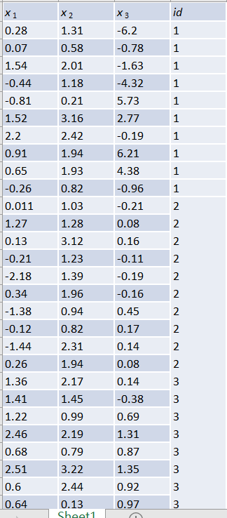
方法二格式如下图，调用集成库，如果数据量大，则用pandas去处理，为了简便代码，就省去了这些

from sklearn.neighbors import KNeighborsClassifier

datas = pd.read_excel('./params2.xlsx', encoding='utf-8')

x1 = np.matrix([0.5,1.0,0.0])
x2 = np.matrix([0.31, 1.51, -0.50])
x3 = np.matrix([-0.3, 0.44, -0.1])

x = datas.drop(['id'], axis=1)
y = datas['id']

knn = KNeighborsClassifier(n_neighbors=5)
knn.fit(x,y)

for i in [1,3,5]:
    for j in [x1, x2, x3]:
        knn = KNeighborsClassifier(n_neighbors=i)
        knn.fit(x,y)
        y_predict = knn.predict(j)
        print("when k={}, the {} belongs to {} ".format(i, j, y_predict))

Outcome:

when k=1, the [[0.5 1.  0. ]] belongs to [2] 
when k=1, the [[ 0.31  1.51 -0.5 ]] belongs to [2] 
when k=1, the [[-0.3   0.44 -0.1 ]] belongs to [2] 
when k=3, the [[0.5 1.  0. ]] belongs to [2] 
when k=3, the [[ 0.31  1.51 -0.5 ]] belongs to [2] 
when k=3, the [[-0.3   0.44 -0.1 ]] belongs to [2] 
when k=5, the [[0.5 1.  0. ]] belongs to [2] 
when k=5, the [[ 0.31  1.51 -0.5 ]] belongs to [2] 
when k=5, the [[-0.3   0.44 -0.1 ]] belongs to [2] 

三. 参考资料

[1] 《机器学习》 周志华
[2] 《模式识别与机器学习》
[3] 利用Python实现kNN算法
[4] 机器学习 —— 基础整理（三）生成式模型的非参数方法： Parzen窗估计、k近邻估计；k近邻分类器
[5] 【机器学习】–非参数估计实验 parzen窗以及k-近邻概率密度——matlab代码
[6] 非参数技术——Parzen窗估计方法

欢迎提出不同的见解~