


原始教程链接:https://github.com/iMetaScience/iMetaPlot/tree/main/221120ggClusterNet-occurrence_network
如果您使用本代码,请引用: Zeyu Zhang. 2022. Tomato microbiome under long-term organic and conventional farming. iMeta 1: e48. 和Tao Wen. 2022. ggClusterNet: An R package for microbiome network analysis and modularity-based multiple network layouts. iMeta 1: e32.
代码编写及注释:农心生信工作室
写在前面
之前我们用较为原始的方法复现过论文中的共现网络,本期我们使用ggClusterNet复现来自中国农业大学李季老师团队的论文Tomato Microbiome under Long-term Organic and Conventional Farming中Figure 4 A-D中的共现网络,Figure 4如下:

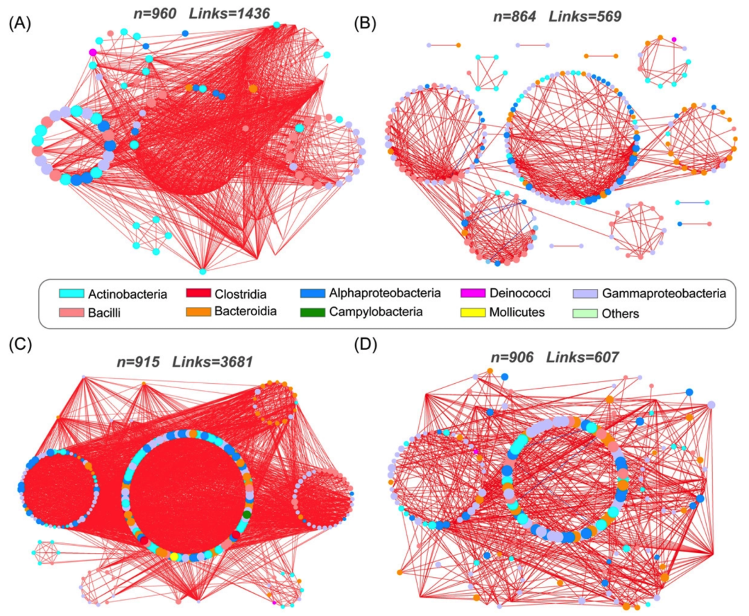
接下来,我们将通过详尽的代码逐步拆解原图,最终实现对原图的复现。
R包检测和安装
01
先安装软件包及其依赖并将所有包载入
# 检查网络图构建包igraph,如没有则安装
if (!require("igraph"))
  install.packages("igraph")
if (!require("BiocManager"))
  install.packages("BiocManager")
if (!require("phyloseq"))
  BiocManager::install("phyloseq")
if (!require("devtools"))
  install.packages("devtools")
if (!require("ggClusterNet"))
  devtools::install_github("taowenmicro/ggClusterNet")
if (!require("ggplot2"))
  install.packages("ggplot2")
if (!require("sna"))
  install.packages("sna")
if (!require("tidyfst"))
  install.packages("tidyfst")


library(igraph)
library(phyloseq)
library(sna)
library(ggClusterNet)
library(ggplot2)
生成测试数据
02
设置随机种子并生成2000个otu的丰度表
# 设置随机数种子,确保数据可重复
set.seed(123)
# 生成A、B两个样本各三个重复,共2000个otu的丰度表
otu <- data.frame(replicate(6, sample.int(10, 2000, replace = T)))
rownames(otu) <- paste0('otu_', 1:nrow(otu)) # 行命名
colnames(otu) <- c('A1', 'A2', 'A3', 'B1', 'B2', 'B3') # 列命名
dim(otu) #查看数据维度
#> [1] 2000    6
# 可选 从文件读取矩阵
# write.table(otu, file = "otu.txt", sep = "\t", quote = F, row.names = T, col.names = T)
# otu = read.table(("otu.txt"), header = T, row.names = 1, sep = "\t", comment.char = "")
03
生成门水平的otu分类并整合数据
otu2tax <- data.frame(row.names = rownames(otu),
                      tax = sample(c('Proteobacteria', 'Firmicutes', 'Acidobacteriota',
                                   'Chloroflexi', 'Verrucomicrobiota', 'Myxococcota',
                                   'Actinobacteriota', 'Gemmatimonadota', 'Latescibacterota'), 2000, replace = T))
# 生成metadata A, B各三个重复
metadata <- data.frame(row.names = colnames(otu),
                       Group = c(rep('A', 3), rep('B', 3)))
# 构建phyloseq对象
ps <- phyloseq(sample_data(metadata),
               otu_table(as.matrix(otu), taxa_are_rows = TRUE),
               tax_table(as.matrix(otu2tax)))
构建图
04
计算OTU之间的相关系数矩阵
result = corMicro(ps = ps,
                  N = 100, # 根据相关系数选取top100进行可视化
                  method.scale = "TMM", # TMM标准化
                  r.threshold = 0.2, # 相关系数阀值
                  p.threshold = 0.05, # p value阀值
                  method = "pearson")
# 提取相关矩阵
cor = result[[1]]
05
构建图
igraph <- graph_from_adjacency_matrix(cor, diag = F, mode="undirected",weighted=TRUE)对节点和边进行注释并分组
06
提取过滤后的OTU表
# 网络中包含的OTU的phyloseq文件提取
ps_net = result[[3]]
# 导出otu表格
otu_table = ps_net %>%
  vegan_otu() %>%
  t() %>%
  as.data.frame()
07
对节点进行注释并随机分为三组
#构建分组,可以根据图的最大连接分组,通过clusters(igraph)得到分组信息;也可以自定义分组,这里随机地将100个过滤后的otu分成三组
gp = data.frame(ID = rownames(otu_table), group = sample(1:3, 100, replace = T))
layout = PolygonClusterG(cor = cor, nodeGroup = gp) # 生成网络图布局,'PolygonClusterG'是该论文中的布局
node = layout[[1]] # 提取节点
tax_table = ps_net %>%
  vegan_tax() %>%
  as.data.frame()
# node节点注释
nodes = nodeadd(plotcord  = node, otu_table = otu_table, tax_table = tax_table)
edge = edgeBuild(cor = cor, node = node)  # 构建边
网络图可视化
08
画图并保存
# 开始绘图
p1 <- ggplot() + geom_segment(data = edge, aes(x = X1, y = Y1, xend = X2, yend = Y2), size = 0.4, color = 'red') +
  geom_point(data = nodes, aes(X1, X2, color = tax), size = 5) +
  scale_colour_brewer(palette = "Set1") +
  scale_size_continuous(range = c(2, 5)) +
  scale_x_continuous(breaks = NULL) + scale_y_continuous(breaks = NULL) +
  theme(panel.background = element_blank()) +
  theme(axis.title.x = element_blank(), axis.title.y = element_blank()) +
  theme(legend.background = element_rect(colour = NA)) +
  theme(panel.background = element_rect(fill = "white",  colour = NA)) +
  theme(panel.grid.minor = element_blank(), panel.grid.major = element_blank())
ggsave("plot.png", p1, width = 10, height = 10) # 保存图片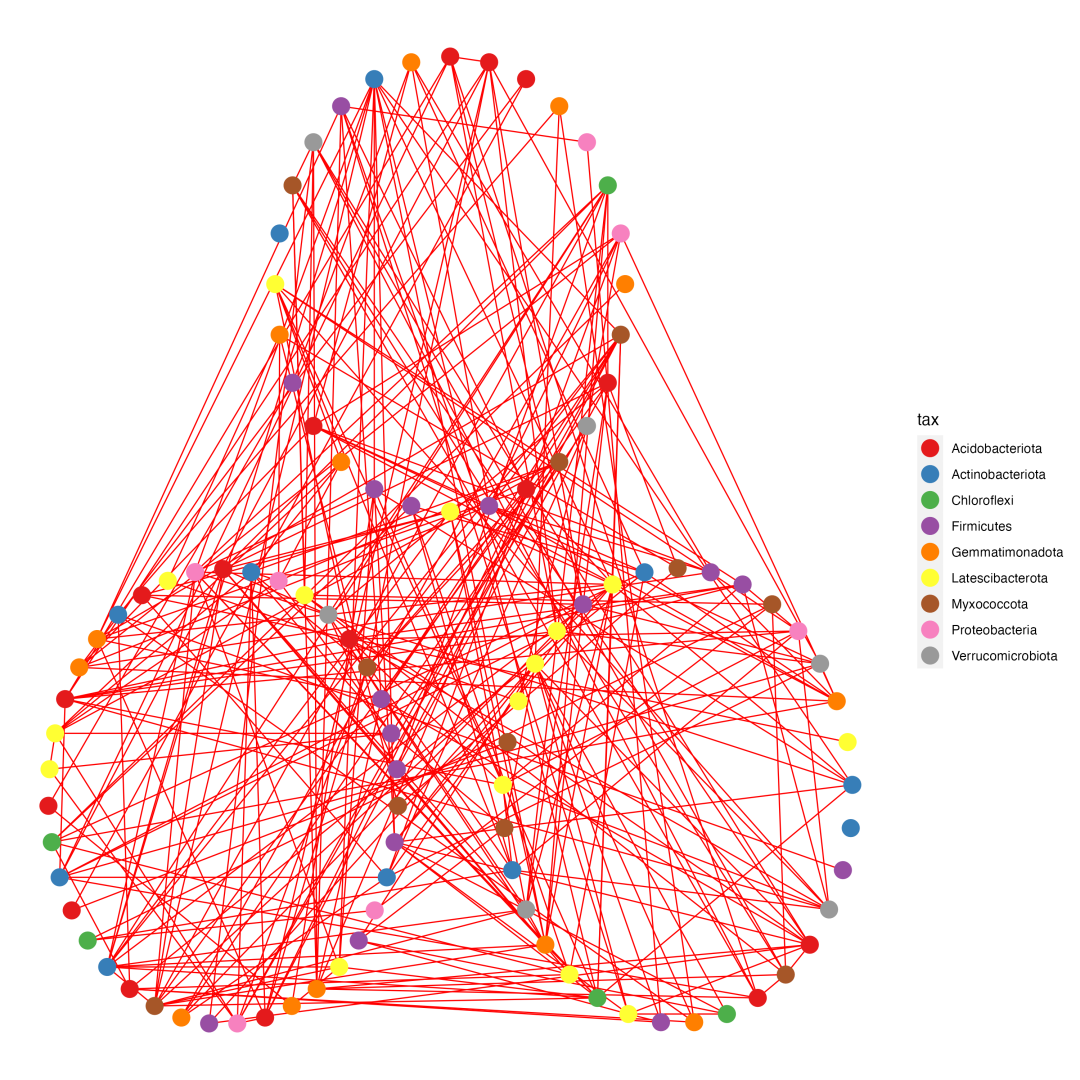
完整代码
# 检查网络图构建包igraph,如没有则安装
if (!require("igraph"))
  install.packages("igraph")
if (!require("BiocManager"))
  install.packages("BiocManager")
if (!require("phyloseq"))
  BiocManager::install("phyloseq")
if (!require("devtools"))
  install.packages("devtools")
if (!require("ggClusterNet"))
  devtools::install_github("taowenmicro/ggClusterNet")
if (!require("ggplot2"))
  install.packages("ggplot2")
if (!require("sna"))
  install.packages("sna")
if (!require("tidyfst"))
  install.packages("tidyfst")


library(igraph)
library(phyloseq)
library(sna)
library(ggClusterNet)
library(ggplot2)


# 设置随机数种子,确保数据可重复
set.seed(123)
# 生成A、B两个样本各三个重复,共2000个otu的丰度表
otu  <-  data.frame(replicate(6, sample.int(10, 2000, replace = T)))
rownames(otu)  <-  paste0('otu_', 1:nrow(otu)) # 行命名
colnames(otu)  <-  c('A1', 'A2', 'A3', 'B1', 'B2', 'B3') # 列命名


dim(otu) #查看数据维度
#> [1] 2000    6


# 可选 从文件读取矩阵
# write.table(otu, file="otu.txt", sep="\t", quote=F, row.names=T, col.names=T)
# otu = read.table(("otu.txt"), header=T, row.names=1, sep="\t", comment.char="")


otu2tax  <-  data.frame(row.names = rownames(otu),
                      tax=sample(c('Proteobacteria', 'Firmicutes', 'Acidobacteriota',
                                   'Chloroflexi', 'Verrucomicrobiota', 'Myxococcota',
                                   'Actinobacteriota', 'Gemmatimonadota', 'Latescibacterota'), 2000, replace = T))
# 生成metadata A, B各三个重复
metadata  <-  data.frame(row.names = colnames(otu),
                       Group=c(rep('A', 3), rep('B', 3)))


# 构建phyloseq对象
ps  <-  phyloseq(sample_data(metadata),
               otu_table(as.matrix(otu), taxa_are_rows=TRUE),
               tax_table(as.matrix(otu2tax)))
result = corMicro(ps = ps,
                  N = 100, # 根据相关系数选取top100进行可视化
                  method.scale = "TMM", # TMM标准化
                  r.threshold=0.2, # 相关系数阀值
                  p.threshold=0.05, # p value阀值
                  method = "pearson")


# 提取相关矩阵
cor = result[[1]]
igraph  <-  graph_from_adjacency_matrix(cor, diag = F, mode="undirected", weighted=TRUE)


# 网络中包含的OTU的phyloseq文件提取
ps_net = result[[3]]


# 导出otu表格
otu_table = ps_net %>%
  vegan_otu() %>%
  t() %>%
  as.data.frame()


#构建分组,可以根据图的最大连接分组,通过clusters(igraph)得到分组信息;也可以自定义分组,这里随机地将100个过滤后的otu分成三组
gp = data.frame(ID = rownames(otu_table), group=sample(1:3, 100, replace = T))
layout = PolygonClusterG(cor = cor, nodeGroup = gp) # 生成网络图布局,'PolygonClusterG'是该论文中的布局
node = layout[[1]] # 提取节点


tax_table = ps_net %>%
  vegan_tax() %>%
  as.data.frame()


# node节点注释
nodes = nodeadd(plotcord =node, otu_table = otu_table, tax_table = tax_table)
edge = edgeBuild(cor = cor, node = node)  # 构建边


# 开始绘图
p1  <-  ggplot() + geom_segment(data = edge, aes(x = X1, y = Y1, xend = X2, yend = Y2), size = 0.4, color = 'red') +
  geom_point(data = nodes, aes(X1, X2, color=tax), size=5) +
  scale_colour_brewer(palette = "Set1") +
  scale_size_continuous(range = c(2, 5)) +
  scale_x_continuous(breaks = NULL) + scale_y_continuous(breaks = NULL) +
  theme(panel.background = element_blank()) +
  theme(axis.title.x = element_blank(), axis.title.y = element_blank()) +
  theme(legend.background = element_rect(colour = NA)) +
  theme(panel.background = element_rect(fill = "white",  colour = NA)) +
  theme(panel.grid.minor = element_blank(), panel.grid.major = element_blank())


ggsave("plot.png", p1, width = 10, height = 10)
以上数据和代码仅供大家参考,如有不完善之处,欢迎大家指正!
更多推荐
(▼ 点击跳转)
iMeta封面 | 宏蛋白质组学分析一站式工具集iMetaLab Suite(加拿大渥太华大学Figeys组)

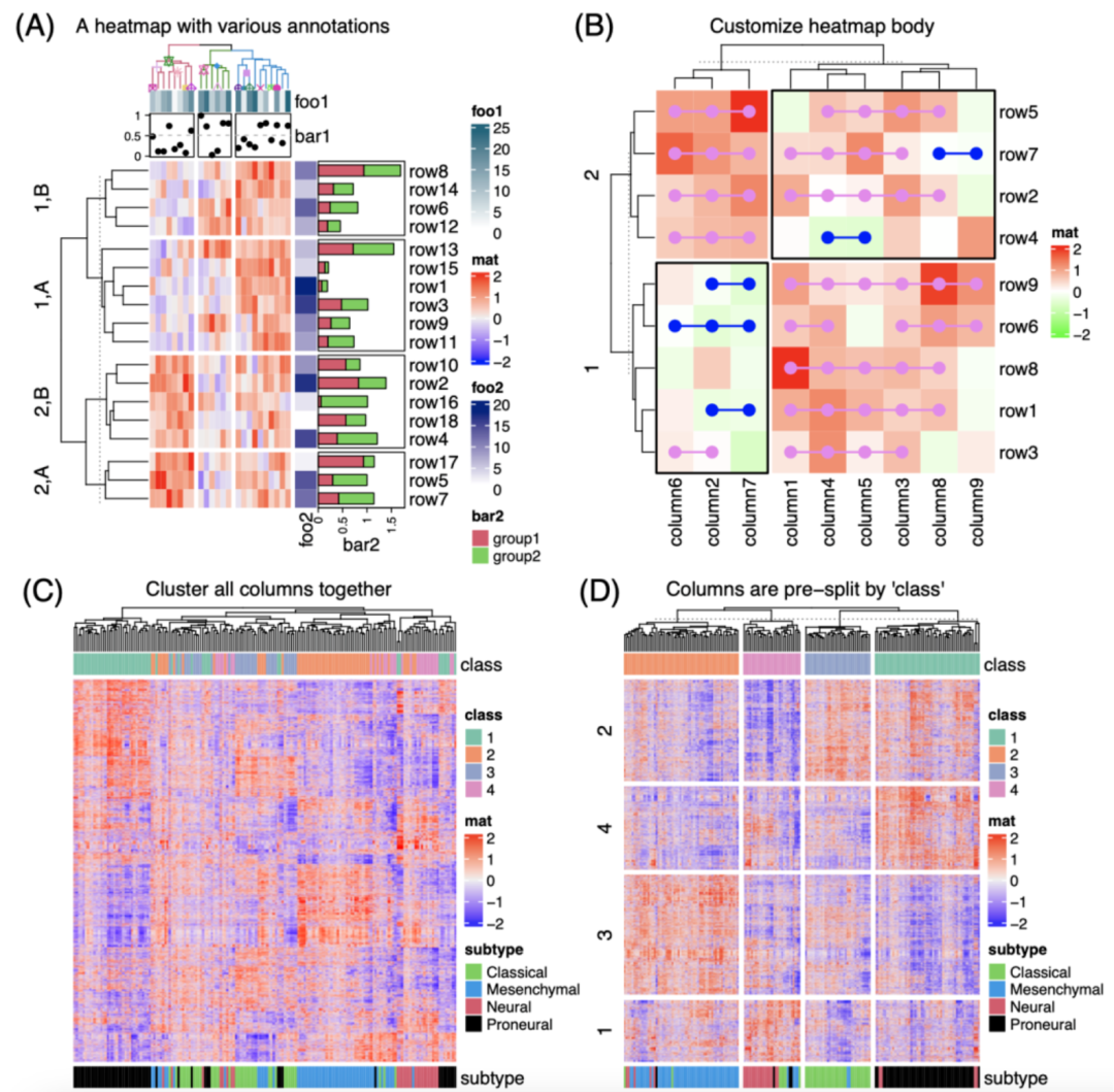
iMeta | 德国国家肿瘤中心顾祖光发表复杂热图(ComplexHeatmap)可视化方法
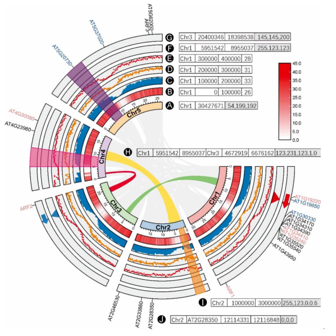
iMeta | 华南农大陈程杰/夏瑞等发布TBtools构造Circos图的简单方法
往期回顾
🔗:https://onlinelibrary.wiley.com/toc/2770596x/2022/1/1

🔗:https://onlinelibrary.wiley.com/toc/2770596x/2022/1/2
期刊简介
“iMeta” 是由威立、肠菌分会和本领域数百位华人科学家合作出版的开放获取期刊,主编由中科院微生物所刘双江研究员和荷兰格罗宁根大学傅静远教授担任。目的是发表原创研究、方法和综述以促进宏基因组学、微生物组和生物信息学发展。目标是发表前10%(IF > 15)的高影响力论文。期刊特色包括视频投稿、可重复分析、图片打磨、青年编委、前3年免出版费、50万用户的社交媒体宣传等。2022年2月正式创刊发行!
联系我们
iMeta主页:http://www.imeta.science
出版社:https://wileyonlinelibrary.com/journal/imeta
投稿:https://mc.manuscriptcentral.com/imeta
邮箱:office@imeta.science
微信公众号
iMeta
责任编辑
微微


 1065
1065

 被折叠的 条评论
为什么被折叠?
被折叠的 条评论
为什么被折叠?
 到【灌水乐园】发言


