SMOTE for Imbalanced Classfication with Python

SMOTE for Imbalanced Classfication with Python

原文地址：https://machinelearningmastery.com/smote-oversampling-for-imbalanced-classification/

不平衡分类主要为，在具有严重类不平衡的数据集上进行开发分类预测模型。如果不处理类不平衡问题，就会导致模型预测性能较差。

其中一种用于处理不平衡数据集的方法是，对小类数据样本进行过采样（oversample）。最简单的方法是将小类数据样本进行复制，尽管复制得到的样本对模型不会增加任何新的信息。

另一种改进的方法，可以从已有样本种合成新样本。这种对于小类样本的数据增强（data augmentation），成为Systhetic Minority Oversampling Technique （SMOTE）。相关论文： Nitesh Chawla, et al. in their 2002 paper named for the technique titled “SMOTE: Synthetic Minority Over-sampling Technique.”

SMOTE选择特征空间中比较接近的样本，在特征空间中的这些样本之间画线，然后，沿着该线画出新的样本。首先，从小类样本中随机选择一个样本a，然后，找寻与之最近地k个近邻（典型的，取k=5）。从中随机选择一个近邻样本b，与样本a构成的特征空间中，创建一个合成的样本。合成的样本是作为样本a和样本b的凸组合。

这种方法可以用于小类样本生成许多合成样本。论文中的建议是，先使用随机降采样来切除大类中一定数量的样本，然后，再使用SMOTE对小类进行过采样来平衡整个数据集。SMOTE和降采样的组合方法优于单单降采样。

这种方法的一个主要缺点，在创建合成样本时没有考虑大类样本，在类与类之间有严重重叠时会导致模棱两可的样本。

Imbalanced-Learn Library

安装 imbalanced-learn Python library

pip install imbalanced-learn

SMOTE for Balancing Data

使用 make_classification() scikit-learn function创建一个合成二分类数据集，样本数位10000，类分布位1：100.

# define dataset
X, y = make_classification(n_samples=10000, n_features=2, n_redundant=0,
	n_clusters_per_class=1, weights=[0.99], flip_y=0, random_state=1)

使用 Counter object 来分析每个类的样本数，确保数据集被正确创建。

# summarize class distribution
counter = Counter(y)
print(counter)

最后，画出数据集的散点图，不同的类采用不同的颜色

# scatter plot of examples by class label
for label, _ in counter.items():
	row_ix = where(y == label)[0]
	pyplot.scatter(X[row_ix, 0], X[row_ix, 1], label=str(label))
pyplot.legend()
pyplot.show()

完整的代码如下：

# Generate and plot a synthetic imbalanced classification dataset
from collections import Counter
from sklearn.datasets import make_classification
from matplotlib import pyplot
from numpy import where
# define dataset
X, y = make_classification(n_samples=10000, n_features=2, n_redundant=0,
	n_clusters_per_class=1, weights=[0.99], flip_y=0, random_state=1)
# summarize class distribution
counter = Counter(y)
print(counter)
# scatter plot of examples by class label
for label, _ in counter.items():
	row_ix = where(y == label)[0]
	pyplot.scatter(X[row_ix, 0], X[row_ix, 1], label=str(label))
pyplot.legend()
pyplot.show()

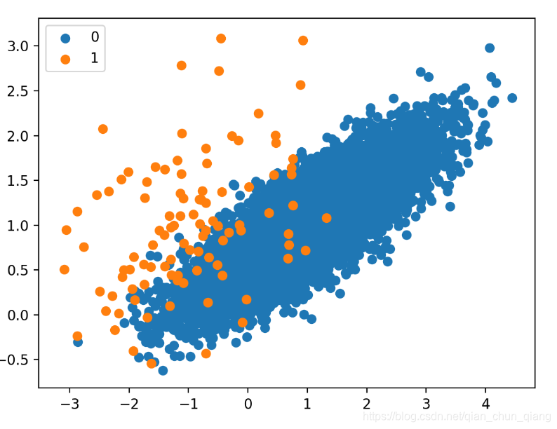
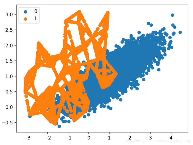
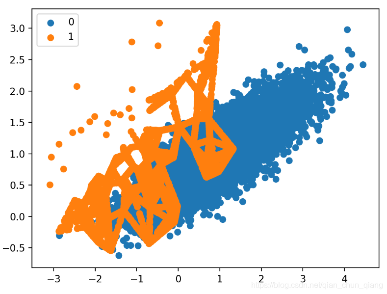
然后，使用SMOTE来过采样小类样本，并画出变换后的数据集。

# Oversample and plot imbalanced dataset with SMOTE
from collections import Counter
from sklearn.datasets import make_classification
from imblearn.over_sampling import SMOTE
from matplotlib import pyplot
from numpy import where
# define dataset
X, y = make_classification(n_samples=10000, n_features=2, n_redundant=0,
	n_clusters_per_class=1, weights=[0.99], flip_y=0, random_state=1)
# summarize class distribution
counter = Counter(y)
print(counter)
# transform the dataset
oversample = SMOTE()
X, y = oversample.fit_resample(X, y)
# summarize the new class distribution
counter = Counter(y)
print(counter)
# scatter plot of examples by class label
for label, _ in counter.items():
	row_ix = where(y == label)[0]
	pyplot.scatter(X[row_ix, 0], X[row_ix, 1], label=str(label))
pyplot.legend()
pyplot.show()

SMOTE的原始论文建议对大类进行随机降采样再结合SMOTE。

RandomUnderSampler class包含随机降采样

我们可以先对小类样本进行过采样至大类样本数量的10%（如，大约1000），然后，使用随机降采样减少大类样本数量至大于小类样本数量50%以上（如，大约2000）。

我们可以定义SMOTE和随机降采样的所需比例系数

over = SMOTE(sampling_strategy=0.1)
under = RandomUnderSampler(sampling_strategy=0.5)

然后，我们可以用Pipeline来组合这两种变换

steps = [('o', over), ('u', under)]
pipeline = Pipeline(steps=steps)

pipeline进行拟合并应用与我们的数据集

# transform the dataset
X, y = pipeline.fit_resample(X, y)

完整的代码

# Oversample with SMOTE and random undersample for imbalanced dataset
from collections import Counter
from sklearn.datasets import make_classification
from imblearn.over_sampling import SMOTE
from imblearn.under_sampling import RandomUnderSampler
from imblearn.pipeline import Pipeline
from matplotlib import pyplot
from numpy import where
# define dataset
X, y = make_classification(n_samples=10000, n_features=2, n_redundant=0,
	n_clusters_per_class=1, weights=[0.99], flip_y=0, random_state=1)
# summarize class distribution
counter = Counter(y)
print(counter)
# define pipeline
over = SMOTE(sampling_strategy=0.1)
under = RandomUnderSampler(sampling_strategy=0.5)
steps = [('o', over), ('u', under)]
pipeline = Pipeline(steps=steps)
# transform the dataset
X, y = pipeline.fit_resample(X, y)
# summarize the new class distribution
counter = Counter(y)
print(counter)
# scatter plot of examples by class label
for label, _ in counter.items():
	row_ix = where(y == label)[0]
	pyplot.scatter(X[row_ix, 0], X[row_ix, 1], label=str(label))
pyplot.legend()
pyplot.show()

SMOTE for Classification

使用先前创建的二分类数据集来拟合和评估决策树算法。

使用默认参数的决策树，使用k-fold cross-validation来评估模型。使用3次重复的10-fold cross-validation，即对数据集拟合和评估30个模型

将数据集分成，即交叉验证的每一折都具有与原始数据集相同的类分布。我们采用 ROC area under curve (AUC) metric评估模型。这种评价比较适合于不平衡数据集有点乐观，但对较好性能模型会仍有相对变化。

# define model
model = DecisionTreeClassifier()
# evaluate pipeline
cv = RepeatedStratifiedKFold(n_splits=10, n_repeats=3, random_state=1)
scores = cross_val_score(model, X, y, scoring='roc_auc', cv=cv, n_jobs=-1)

拟合之后，我们可以计算平均分数

print('Mean ROC AUC: %.3f' % mean(scores))

我们不会期待决策树能对原始数据集表现得很好，完整的代码如下

# decision tree evaluated on imbalanced dataset
from numpy import mean
from sklearn.datasets import make_classification
from sklearn.model_selection import cross_val_score
from sklearn.model_selection import RepeatedStratifiedKFold
from sklearn.tree import DecisionTreeClassifier
# define dataset
X, y = make_classification(n_samples=10000, n_features=2, n_redundant=0,
	n_clusters_per_class=1, weights=[0.99], flip_y=0, random_state=1)
# define model
model = DecisionTreeClassifier()
# evaluate pipeline
cv = RepeatedStratifiedKFold(n_splits=10, n_repeats=3, random_state=1)
scores = cross_val_score(model, X, y, scoring='roc_auc', cv=cv, n_jobs=-1)
print('Mean ROC AUC: %.3f' % mean(scores))

得到的结果为

Mean ROC AUC: 0.761

现在，我们使用相同的模型和评估方法，但使用SMOTE变换后的数据集。

在k折交叉验证时进行正确的过采样处理，则SMOTE方法只能应用在训练集上，然后用没有变换过的测试集来评估模型。

可以设置pipeline来首先对训练集SMOTE变换，然后训练模型

# define pipeline
steps = [('over', SMOTE()), ('model', DecisionTreeClassifier())]
pipeline = Pipeline(steps=steps)

这个pipeline可以用重复k折交叉验证来评估

完整的代码如下

# decision tree evaluated on imbalanced dataset with SMOTE oversampling
from numpy import mean
from sklearn.datasets import make_classification
from sklearn.model_selection import cross_val_score
from sklearn.model_selection import RepeatedStratifiedKFold
from sklearn.tree import DecisionTreeClassifier
from imblearn.pipeline import Pipeline
from imblearn.over_sampling import SMOTE
# define dataset
X, y = make_classification(n_samples=10000, n_features=2, n_redundant=0,
	n_clusters_per_class=1, weights=[0.99], flip_y=0, random_state=1)
# define pipeline
steps = [('over', SMOTE()), ('model', DecisionTreeClassifier())]
pipeline = Pipeline(steps=steps)
# evaluate pipeline
cv = RepeatedStratifiedKFold(n_splits=10, n_repeats=3, random_state=1)
scores = cross_val_score(pipeline, X, y, scoring='roc_auc', cv=cv, n_jobs=-1)
print('Mean ROC AUC: %.3f' % mean(scores))

运行结果为

Mean ROC AUC: 0.809

算法文献中提到，SMOTE在对大类进行降采样（如，随机降采样）时会表现得更好

我们可以在pipeline中简单增加RandomUnderSampler 步骤

正如上一节提到得，我们先对小类别样本以系数1：10进行SMOTE进行过采样，然后对大类别样本进行降采样之1：2.

# define pipeline
model = DecisionTreeClassifier()
over = SMOTE(sampling_strategy=0.1)
under = RandomUnderSampler(sampling_strategy=0.5)
steps = [('over', over), ('under', under), ('model', model)]
pipeline = Pipeline(steps=steps)

完整的代码

# decision tree  on imbalanced dataset with SMOTE oversampling and random undersampling
from numpy import mean
from sklearn.datasets import make_classification
from sklearn.model_selection import cross_val_score
from sklearn.model_selection import RepeatedStratifiedKFold
from sklearn.tree import DecisionTreeClassifier
from imblearn.pipeline import Pipeline
from imblearn.over_sampling import SMOTE
from imblearn.under_sampling import RandomUnderSampler
# define dataset
X, y = make_classification(n_samples=10000, n_features=2, n_redundant=0,
	n_clusters_per_class=1, weights=[0.99], flip_y=0, random_state=1)
# define pipeline
model = DecisionTreeClassifier()
over = SMOTE(sampling_strategy=0.1)
under = RandomUnderSampler(sampling_strategy=0.5)
steps = [('over', over), ('under', under), ('model', model)]
pipeline = Pipeline(steps=steps)
# evaluate pipeline
cv = RepeatedStratifiedKFold(n_splits=10, n_repeats=3, random_state=1)
scores = cross_val_score(pipeline, X, y, scoring='roc_auc', cv=cv, n_jobs=-1)
print('Mean ROC AUC: %.3f' % mean(scores))

运行结果

Mean ROC AUC: 0.834

你可以探索测试不同小类别和大类别的比例系数（如，改变sampling_strategy参数），看模型性能是否有所改善。

另外一个方面可探索的是，在SMOTE步骤合成每个新样本时，选择k近邻的不同k值。默认的k值为5，该值的变大或变小会影响所生成的样本的类型，并且会影响模型的性能。

例如，我们可以采用对k值进行grid search，比如值从1至7，并评估每个值下的pipeline。

...
# values to evaluate
k_values = [1, 2, 3, 4, 5, 6, 7]
for k in k_values:
	# define pipeline

完整的代码

# grid search k value for SMOTE oversampling for imbalanced classification
from numpy import mean
from sklearn.datasets import make_classification
from sklearn.model_selection import cross_val_score
from sklearn.model_selection import RepeatedStratifiedKFold
from sklearn.tree import DecisionTreeClassifier
from imblearn.pipeline import Pipeline
from imblearn.over_sampling import SMOTE
from imblearn.under_sampling import RandomUnderSampler
# define dataset
X, y = make_classification(n_samples=10000, n_features=2, n_redundant=0,
	n_clusters_per_class=1, weights=[0.99], flip_y=0, random_state=1)
# values to evaluate
k_values = [1, 2, 3, 4, 5, 6, 7]
for k in k_values:
	# define pipeline
	model = DecisionTreeClassifier()
	over = SMOTE(sampling_strategy=0.1, k_neighbors=k)
	under = RandomUnderSampler(sampling_strategy=0.5)
	steps = [('over', over), ('under', under), ('model', model)]
	pipeline = Pipeline(steps=steps)
	# evaluate pipeline
	cv = RepeatedStratifiedKFold(n_splits=10, n_repeats=3, random_state=1)
	scores = cross_val_score(pipeline, X, y, scoring='roc_auc', cv=cv, n_jobs=-1)
	score = mean(scores)
	print('> k=%d, Mean ROC AUC: %.3f' % (k, score))

运行结果

> k=1, Mean ROC AUC: 0.827
> k=2, Mean ROC AUC: 0.823
> k=3, Mean ROC AUC: 0.834
> k=4, Mean ROC AUC: 0.840
> k=5, Mean ROC AUC: 0.839
> k=6, Mean ROC AUC: 0.839
> k=7, Mean ROC AUC: 0.853

这表明，过采样数量和降采样的策略，以及从多少个样本中选择并合成新样本（k_neighbors）可能都是对你所用的数据集的选择和调节的重要参数。

SMOTE With Selective Synthetic Sample Generation

这一节，我们将回顾一些SMOTE的扩展，基于小类别样本更具选择性以给出产生新合成样本的基础。

Borderline-SMOTE

其中一个比较流行的扩展是，选择那些小类别中被误分类的样本（如，k近邻分类模型）。

然后，我们只对那些困难的样本进行过采样，只对那些较高分辨率的地方处理。

文献 Borderline-SMOTE: A New Over-Sampling Method in Imbalanced Data Sets Learning, 2005.中指出，靠近边界线上的那些样本比远离边界线的那些更容易被误分类，因此对于分类来说更重要。

这些样本被误分类很可能是因为模棱两可。即，决策边界附近的不同类样本会有相互重叠。

文献作者描述了被包含在大类别中导致小类别的边界线处的误分类的样本进行过采样的方法–Borderline-SMOTE1；只对小类别边界处的样本进行过采样的方法—Borderline-SMOTE2.

Borderline-SMOTE2不仅对处于DANGER中的每个样本产生合成样本，并且正近邻的为P，同时负最近邻为N。

这里，我们不再只是盲目地对小类别样本产生新的合成样本，而是期待Borderline-SMOTE方法只对沿着两个类别之间的决策边界进行生产合成样本。

使用Borderline-SMOTE方法进行过采样二分类数据集的完整代码如下

# borderline-SMOTE for imbalanced dataset
from collections import Counter
from sklearn.datasets import make_classification
from imblearn.over_sampling import BorderlineSMOTE
from matplotlib import pyplot
from numpy import where
# define dataset
X, y = make_classification(n_samples=10000, n_features=2, n_redundant=0,
	n_clusters_per_class=1, weights=[0.99], flip_y=0, random_state=1)
# summarize class distribution
counter = Counter(y)
print(counter)
# transform the dataset
oversample = BorderlineSMOTE()
X, y = oversample.fit_resample(X, y)
# summarize the new class distribution
counter = Counter(y)
print(counter)
# scatter plot of examples by class label
for label, _ in counter.items():
	row_ix = where(y == label)[0]
	pyplot.scatter(X[row_ix, 0], X[row_ix, 1], label=str(label))
pyplot.legend()
pyplot.show()

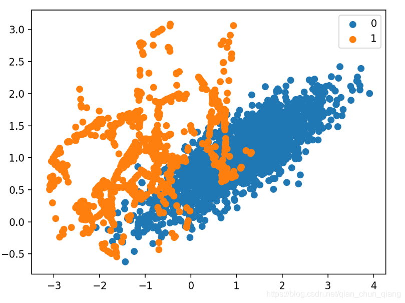
变换后的数据集的散点图如下图所示。可以清楚地看到选择性地过采样地效果。沿着决策边界的小类别样本被着重过采样。

而那些远离决策边界的样本则没有被过采样。这包括那些容易分类的样本，以及那些及其难以分类的样本

Borderline-SMOTE SVM

Hien Nguyen等人建议使用另一种Borderline-SMOTE形式，即用SVM来代替KNN进行在决策边界处的误分类样本的辨别。

他们的方法总结在2009年的那篇文献 “Borderline Over-sampling For Imbalanced Data Classification.” SVM用来确定由support vectors定义的决策边界位置。小类别中靠近support vectors的那些样本被重点进行产生合成样本

在对原始训练集对标准SVM分类器进行训练得到由support vectors近似的边界线区域。并对一定数量的最近邻的每个小类别样本的support vector进行插值成线，沿着线随机生成新的样本。

除了使用SVM，该技术还尝试选择那些较少小类别样本的区域，并试着朝类边界进行外推。

如果主要类别的数量小于其近邻数量的一半，则采用从小类别区域外推只主类别来生成新样本。

完整的代码

# borderline-SMOTE with SVM for imbalanced dataset
from collections import Counter
from sklearn.datasets import make_classification
from imblearn.over_sampling import SVMSMOTE
from matplotlib import pyplot
from numpy import where
# define dataset
X, y = make_classification(n_samples=10000, n_features=2, n_redundant=0,
	n_clusters_per_class=1, weights=[0.99], flip_y=0, random_state=1)
# summarize class distribution
counter = Counter(y)
print(counter)
# transform the dataset
oversample = SVMSMOTE()
X, y = oversample.fit_resample(X, y)
# summarize the new class distribution
counter = Counter(y)
print(counter)
# scatter plot of examples by class label
for label, _ in counter.items():
	row_ix = where(y == label)[0]
	pyplot.scatter(X[row_ix, 0], X[row_ix, 1], label=str(label))
pyplot.legend()
pyplot.show()

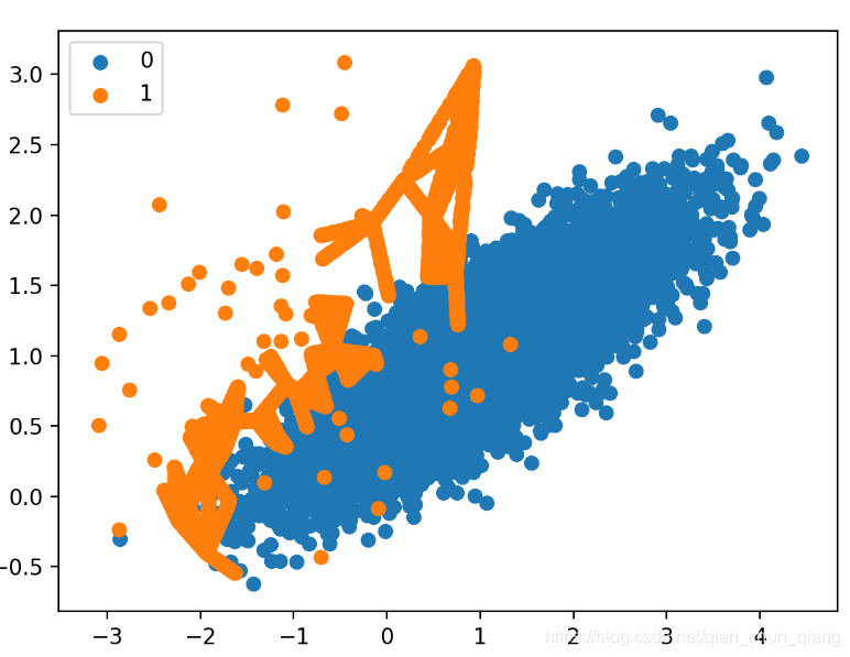
变换后的数据集离散图显示，沿着伴有主类别的决策边界进行直接过采样。同时，不同于Borderline-SMOTE，在远离类重叠区域处也合成了更多的样本，如图中左上部分。

Adaptive Synthetic Sampling (ADASYN)

另一种方法，生成的合成样本与小类别样本在该处的密度成反比。

也就是说，在小类别样本密度较低的特征空间区域生成更多合成样本，而在密度较高的地方则少生成合成样本。

该方法由Haibo He等人提出的，2008年的文献“ADASYN: Adaptive Synthetic Sampling Approach For Imbalanced Learning.”

该方法的关键思想为，使用密度分布作为自动决策对每个小类别样本所需的合成样本数量。

完成的代码如下

# Oversample and plot imbalanced dataset with ADASYN
from collections import Counter
from sklearn.datasets import make_classification
from imblearn.over_sampling import ADASYN
from matplotlib import pyplot
from numpy import where
# define dataset
X, y = make_classification(n_samples=10000, n_features=2, n_redundant=0,
	n_clusters_per_class=1, weights=[0.99], flip_y=0, random_state=1)
# summarize class distribution
counter = Counter(y)
print(counter)
# transform the dataset
oversample = ADASYN()
X, y = oversample.fit_resample(X, y)
# summarize the new class distribution
counter = Counter(y)
print(counter)
# scatter plot of examples by class label
for label, _ in counter.items():
	row_ix = where(y == label)[0]
	pyplot.scatter(X[row_ix, 0], X[row_ix, 1], label=str(label))
pyplot.legend()
pyplot.show()

从变换后的数据集的散点图可以看出，类似Borderline-SMOTE，合成样本的产生主要集中在决策边界的具有较低密度的区域。

而与Borderline-SMOTE相区别的是，在最大类别重叠的样本被受到最大的关注。对于这一类的低密度样本可能为异常样本。因此，ADASYN方法可能对特征空间的这些区域关注太多，可能使模型的性能变差。

可能在应用过采样步骤前，最好先进行异常样本的移除。

Further Reading

This section provides more resources on the topic if you are looking to go deeper.

Books

• Learning from Imbalanced Data Sets, 2018.
• Imbalanced Learning: Foundations, Algorithms, and Applications, 2013.

Papers

• SMOTE: Synthetic Minority Over-sampling Technique, 2002.
• Borderline-SMOTE: A New Over-Sampling Method in Imbalanced Data Sets Learning, 2005.
• Borderline Over-sampling For Imbalanced Data Classification, 2009.
• ADASYN: Adaptive Synthetic Sampling Approach For Imbalanced Learning, 2008.

API

• imblearn.over_sampling.SMOTE API.
• imblearn.over_sampling.SMOTENC API.
• imblearn.over_sampling.BorderlineSMOTE API.
• imblearn.over_sampling.SVMSMOTE API.
• imblearn.over_sampling.ADASYN API.

Articles

https://imbalanced-learn.readthedocs.io/en/stable/generated/imblearn.over_sampling.SMOTENC.html).

• imblearn.over_sampling.BorderlineSMOTE API.
• imblearn.over_sampling.SVMSMOTE API.
• imblearn.over_sampling.ADASYN API.

Articles

• Oversampling and undersampling in data analysis, Wikipedia.