


文章目录
介绍
翻译自pytorch目标检测教程,并提供了双语版本。
开发环境
- Pytorch 0.4
- Python 3.6
Objective(目标)
To build a model that can detect and localize specific objects in images.
创建一个用来检测和定位图片中特定物体的模型
We will be implementing the Single Shot Multibox Detector (SSD).The authors’ original implementation can be found here.
我们将要实现SSD(Single Shot Multibox Detector )检测器
Concepts(概念)
-
Object Detection. duh.
-
Single-Shot Detection(SSD). Earlier architectures for object detection consisted of two distinct stages – a region proposal network that performs object localization and a classifier for detecting the types of objects in the proposed regions. Computationally, these can be very expensive and therefore ill-suited for real-world, real-time applications. Single-shot models encapsulate(压缩) both localization and detection tasks in a single forward sweep of the network, resulting in significantly faster detections while deployable on lighter hardware.
(SSD:早期的目标检测包括两个不同的阶段——一个是执行定位的区域提议网络 ,另一个是检测提议区域内物体类别的分类器,但是他们计算花销时很大的,并且不适合真实世界里的实时应用,SSD将定位和预测任务压缩到网络的一个前向传播中,这使得在轻量的硬件中,它能够以相当快的速度进行检测) -
Multiscale Feature Maps. In image classification tasks, we base our predictions on the final convolutional feature map – the smallest but deepest representation of the original image. In object detection, feature maps from intermediate convolutional layers can also be directly useful because they represent the original image at different scales. Therefore, a fixed-size filter operating on different feature maps will be able to detect objects of various sizes.
(多尺度特征图:在图像分类任务中,我们的预测依据的是最终的卷积特征图,即原图像在网络中最小、最深的描述。在目标检测中,处于中间卷积层的特征图同样是有用的,因为他们代表了原图像的不同尺度。因为,当一个固定大小的滤波器作用在不同的特征图上时,就可以检测到不同大小的物体。) -
Priors. These are pre-computed boxes defined at specific positions on specific feature maps, with specific aspect ratios and scales. They are carefully chosen to match the characteristics of objects’ bounding boxes (i.e. the ground truths) in the dataset.
(先验:这是一些在特定特征图的特定位置预先计算的框,这些框有特定的比例系数和宽高比,我们需要小心的选出他们来匹配数据集中物体的边界框特征) -
Multibox. This is a technique that formulates predicting an object’s bounding box as a regression problem, wherein a detected object’s coordinates are regressed to its ground truth’s coordinates. In addition, for each predicted box, scores are generated for various object types. Priors serve as feasible starting points for predictions because they are modeled on the ground truths. Therefore, there will be as many predicted boxes as there are priors, most of whom will contain no object.
(Multibox:这是一种将预测对象的边界框作为回归问题的技术,) -
Hard Negative Mining. This refers to(指的是) explicitly(明确的) choosing the most egregious(过分的) false positives predicted by a model and forcing it to learn from these examples. In other words, we are mining only those negatives that the model found hardest to identify correctly. In the context of object detection, where the vast majority of (绝大部分)predicted boxes do not contain an object, this also serves to reduce the negative-positive imbalance.
(难分样本挖掘:这指的是,找出模型中明显的被模型预测为正的负样本(FP),并使模型去学习这个例子。换句话说,我们只是在挖掘那些模型难以正确识别的负面信息,在目标检测中,其中绝大多数预测框不包含对象,这也有助于减少正负不平衡) -
Non-Maximum Suppression. At any given location, multiple priors can overlap significantly(相当数量地). Therefore, predictions arising out of these priors(由这些先验得出的预测) could actually be duplicates of the same object. Non-Maximum Suppression (NMS) is a means to remove redundant predictions by suppressing all but the one with the maximum score.
(非极大值抑制:任意给定的一个位置,可能有多个先验框覆盖它,因此,由这些先验得出的预测会产生重复,非极大值抑制就是一种通过抑制除了拥有最大得分以外的其他点来去除冗余预测的方法)
Overview(综述)
As we proceed, you will notice that there’s a fair bit of (不少的)engineering that’s resulted in the SSD’s very specific structure and formulation. Don’t worry if some aspects of it seem contrived or unspontaneous at first. Remember, it’s built upon years of (often empirical) research in this field.
随着我们的进展,你会注意到有相当多的工程技巧导致了SSD特定的结构和公式。不要担心,在你刚开始学习的时候,如果它的某些方面看起来不自然。请记住,它是建立在这个领域多年(通常是经验主义的)研究基础上的。
Some definitions(一些定义)
A box is a box. A bounding box is a box that wraps around an object i.e. represents its bounds.
In this tutorial, we will encounter both types – just boxes and bounding boxes. But all boxes are represented on images and we need to be able to measure their positions, shapes, sizes, and other properties.
- Boundary coordinates
The most obvious way to represent a box is by the pixel coordinates of the x and y lines that constitute its boundaries.
![[外链图片转存失败,源站可能有防盗链机制,建议将图片保存下来直接上传(img-tCy9K3qf-1581996372296)(https://github.com/sgrvinod/a-PyTorch-Tutorial-to-Object-Detection/raw/master/img/bc1.PNG)]](https://img-blog.csdnimg.cn/20200218112641722.png?x-oss-process=image/watermark,type_ZmFuZ3poZW5naGVpdGk,shadow_10,text_aHR0cHM6Ly9ibG9nLmNzZG4ubmV0L3FpYW9fcWlhb19kZV9mZW5nX2xl,size_16,color_FFFFFF,t_70)
The boundary coordinates of a box are simply (x_min, y_min, x_max, y_max).
But pixel values are next to useless if we don’t know the actual dimensions of the image. A better way would be to represent all coordinates is in their fractional(分数的、小数的) form.

Now the coordinates are size-invariant and all boxes across all images are measured on the same scale.
(现在所有的坐标都是大小相同的,并且不同图片上的框能够通过相同的尺度来度量) - Center-Size coordinates
This is a more explicit way of representing a box’s position and dimensions.

The center-size coordinates of a box are (c_x, c_y, w, h).
In the code, you will find that we routinely use both coordinate systems depending upon their suitability for the task, and always in their fractional forms. - Jaccard Index(jaccard指数)
The Jaccard Index or Jaccard Overlap or Intersection-over-Union (IoU) measure the degree or extent to which two boxes overlap
(Jaccard系数或交并比(IoU)度量两个盒子重叠的程度)

An IoU of 1 implies they are the same box, while a value of 0 indicates they’re mutually(相互) exclusive(独立的) spaces.
It’s a simple metric(度量标准), but also one that finds many applications in our mode
Multibox
Multibox is a technique for detecting objects where a prediction consists of two components
- Coordinates of a box that may or may not contain an object. This is a regression task.(回归任务)
- Scores for various object types for this box, including a background class which implies there is no object in the box. This is a classification task.(分类任务)
Single Shot Detector (SSD)
The SSD is a purely convolutional neural network (CNN) that we can organize into three parts
- Base convolutions derived from an existing image classification architecture that will provide lower-level feature maps.
- Auxiliary convolutions added on top of the base network that will provide higher-level feature maps.
- Prediction convolutions that will locate and identify objects in these feature maps.
The paper demonstrates two variants of the model called the SSD300 and the SSD512. The suffixes(后缀) represent the size of the input image. Although the two networks differ slightly in the way they are constructed, they are in principle the same. The SSD512 is just a larger network and results in marginally better performance.
For convenience, we will deal with the SSD300.
Base Convolutions – part 1
First of all, why use convolutions from an existing network architecture?
Because models proven to work well with image classification are already pretty good at capturing the basic essence of(主要的构成要件) an image. The same convolutional features are useful for object detection, albeit in a more local sense – we’re less interested in the image as a whole than specific regions of it where objects are present.
(因为已经被证明可以很好的进行图像分类的模型可以很好的捕捉图像的主要构成要素。相同的卷积特性对于目标检测也很有用,尽管是在更局部的意义上,比起整幅图像,我们对目标存在的特定区域更加感兴趣)
There’s also the added advantage of being able to use layers pretrained on a reliable classification dataset. As you may know, this is called Transfer Learning. By borrowing knowledge from a different but closely related task, we’ve made progress before we’ve even begun.
(使用已经在一个可靠的数据集上训练好的模型也会有很多其优势,这就是迁移学习。通过借用一个不同但相近任务的知识,我们可以在还没有开始训练情况下就取得一定的进展)
The authors of the paper employ the VGG-16 architecture as their base network. It’s rather simple in its original form.

They recommend using one that’s pretrained on the ImageNet Large Scale Visual Recognition Competition (ILSVRC) classification task. Luckily, there’s one already available in PyTorch, as are other popular architectures. If you wish, you could opt for something larger like the ResNet. Just be mindful of(注意) the computational requirements.
As per the paper, we’ve to make some changes to this pretrained network to adapt it to our own challenge of object detection. Some are logical and necessary, while others are mostly a matter of convenience or preference.
(我们需要修改这个训练好的模型让他更加适合我们的目标检测工作,这些改动中,一些是符合逻辑并且必要的,另外一些则是为了方便或者说是作者的偏好)
-
The input image size will be 300, 300, as stated earlier.
(输入图像的大小是300*300) -
The 3rd pooling layer, which halves dimensions, will use the mathematical ceiling function instead of the default floor function in determining output size. This is significant only if the dimensions of the preceding feature map are odd and not even. By looking at the image above, you could calculate that for our input image size of 300, 300, the conv3_3 feature map will be of cross-section 75, 75, which is halved to 38, 38 instead of an inconvenient 37, 37.
-
We modify the 5th pooling layer from a 2, 2 kernel and 2 stride to a 3, 3 kernel and 1 stride. The effect this has is it no longer halves the dimensions of the feature map from the preceding convolutional layer.
-
We don’t need the fully connected (i.e. classification) layers because they serve no purpose here. We will toss fc8 away completely, but choose to rework fc6 and fc7 into convolutional layers conv6 and conv7.
The first three modifications are straightforward enough, but that last one probably needs some explaining.
FC → Convolutional Layer
How do we reparameterize a fully connected layer into a convolutional layer?
Consider the following scenario(设想).
In the typical image classification setting, the first fully connected layer cannot operate on the preceding feature map or image directly. We’d need to flatten it into a 1D structure.

In this example, there’s an image of dimensions 2, 2, 3, flattened to a 1D vector of size 12. For an output of size 2, the fully connected layer computes two dot-products of this flattened image with two vectors of the same size 12. These two vectors, shown in gray, are the parameters of the fully connected layer.
Now, consider a different scenario where we use a convolutional layer to produce 2 output values.

Here, the image of dimensions 2, 2, 3 need not be flattened, obviously. The convolutional layer uses two filters with 12 elements in the same shape as the image to perform two dot products. These two filters, shown in gray, are the parameters of the convolutional layer.
But here’s the key part – in both scenarios, the outputs Y_0 and Y_1 are the same!

The two scenarios are equivalent.
What does this tell us?
That on an image of size H, W with I input channels, a fully connected layer of output size N is equivalent to a convolutional layer with kernel size equal to the image size H, W and N output channels, provided that the parameters of the fully connected network N, H * W * I are the same as the parameters of the convolutional layer N, H, W, I.

Therefore, any fully connected layer can be converted to an equivalent convolutional layer simply by reshaping its parameters.
(因此,任何全连接层都可以通过改变参数的形状被转换为等价的卷积层)
Base Convolutions – part 2
We now know how to convert fc6 and fc7 in the original VGG-16 architecture into conv6 and conv7 respectively.
In the ImageNet VGG-16 shown previously, which operates on images of size 224, 224, 3, you can see that the output of conv5_3 will be of size 7, 7, 512. Therefore –
-
fc6 with a flattened input size of 7 * 7 * 512 and an output size of 4096 has parameters of dimensions 4096, 7 * 7 * 512. The equivalent convolutional layer conv6 has a 7, 7 kernel size and 4096 output channels, with reshaped parameters of dimensions 4096, 7, 7, 512.
-
fc7 with an input size of 4096 (i.e. the output size of fc6) and an output size 4096 has parameters of dimensions 4096, 4096. The input could be considered as a 1, 1 image with 4096 input channels. The equivalent convolutional layer conv7 has a 1, 1 kernel size and 4096 output channels, with reshaped parameters of dimensions 4096, 1, 1, 4096.
We can see that conv6 has 4096 filters, each with dimensions 7, 7, 512, and conv7 has 4096 filters, each with dimensions 1, 1, 4096.
These filters are numerous and large – and computationally expensive.
To remedy(补救) this, the authors opt to reduce both their number and the size of each filter by subsampling parameters from the converted convolutional layers.
-
conv6 will use 1024 filters, each with dimensions 3, 3, 512. Therefore, the parameters are subsampled from 4096, 7, 7, 512 to 1024, 3, 3, 512.
-
conv7 will use 1024 filters, each with dimensions 1, 1, 1024. Therefore, the parameters are subsampled from 4096, 1, 1, 4096 to 1024, 1, 1, 1024.
Based on the references in the paper, we will subsample by picking every mth parameter along a particular dimension, in a process known as decimation.
Since the kernel of conv6 is decimated from 7, 7 to 3, 3 by keeping only every 3rd value, there are now holes in the kernel. Therefore, we would need to make the kernel dilated or atrous.
This corresponds to a dilation of 3 (same as the decimation factor m = 3). However, the authors actually use a dilation of 6, possibly because the 5th pooling layer no longer halves the dimensions of the preceding feature map.
We are now in a position to present our base network, the modified VGG-16.

In the above figure, pay special attention to the outputs of conv4_3 and conv_7. You will see why soon enough.
Auxiliary Convolutions
We will now stack some more convolutional layers on top of our base network. These convolutions provide additional feature maps, each progressively(逐渐的) smaller than the last.

We introduce four convolutional blocks, each with two layers. While size reduction happened through pooling in the base network, here it is facilitated by a stride of 2 in every second layer.
Again, take note of the feature maps from conv8_2, conv9_2, conv10_2, and conv11_2.
A detour(稍微思考一下)
Before we move on to the prediction convolutions, we must first understand what it is we are predicting. Sure, it’s objects and their positions, but in what form?
(在我们实现预测卷积之前,我们必须知道我们在预测什么。——我们预测的是目标和它的位置,但是是以什么形式来预测呢?)
It is here that we must learn about priors and the crucial role they play in the SSD.
(我们必须先要了解Prior以及它在SSD中所扮演的角色)
Priors
Object predictions can be quite diverse(多种多样), and I don’t just mean their type. They can occur at any position, with any size and shape. Mind you(注意), we shouldn’t go as far as to say there are infinite possibilities for where and how an object can occur. While this may be true mathematically, many options are simply improbable or uninteresting. Furthermore, we needn’t insist that boxes are pixel-perfect.
In effect(实际上), we can discretize(离散化) the mathematical space of potential predictions into just thousands of possibilities.
Priors are precalculated, fixed boxes which collectively (公共)represent this universe of probable and approximate box predictions.
(Priors 是预先计算好的,固定的方框,它们共同代表了可能的全集和近似的预测框。)。
Priors are manually but carefully chosen based on the shapes and sizes of ground truth objects in our dataset. By placing these priors at every possible location in a feature map, we also account for variety in position.
(Priors是人为选出的,它基于数据集中目标真值的形状和大小。我们通过把这些priors放在特征图的每个可能位置来考虑位置的多样性)
In defining the priors, the authors specify that –
-
they will be applied to various low-level and high-level feature maps, viz(即). those from conv4_3, conv7, conv8_2, conv9_2, conv10_2, and conv11_2. These are the same feature maps indicated on the figures before.
-
if a prior has a scale s, then its area is equal to that of a square with side s. The largest feature map, conv4_3, will have priors with a scale of 0.1, i.e. 10% of image’s dimensions, while the rest have priors with scales linearly increasing from 0.2 to 0.9. As you can see, larger feature maps have priors with smaller scales and are therefore ideal for detecting smaller objects.
-
At each position on a feature map, there will be priors of various aspect ratios. All feature maps will have priors with ratios 1:1, 2:1, 1:2. The intermediate feature maps of conv7, conv8_2, and conv9_2 will also have priors with ratios 3:1, 1:3. Moreover, all feature maps will have one extra prior with an aspect ratio of 1:1 and at a scale that is the geometric mean of the scales of the current and subsequent feature map.
-

-
There are a total of 8732 priors defined for the SSD300!
Visualizing Priors
We defined the priors in terms of their scales and aspect ratios.

Solving these equations yields a prior’s dimensions w and h.

We’re now in a position to draw them on their respective feature maps.
For example, let’s try to visualize what the priors will look like at the central tile of the feature map from conv9_2.

The same priors also exist for each of the other tiles.

Predictions vis-à-vis Priors
Earlier, we said we would use regression to find the coordinates of an object’s bounding box. But then, surely, the priors can’t represent our final predicted boxes?
They don’t.
Again, I would like to reiterate(重申) that the priors represent, approximately, the possibilities for prediction.
(priors近似地代表预测的可能性)
This means that we use each prior as an approximate starting point and then find out how much it needs to be adjusted to obtain a more exact prediction for a bounding box.
(这意味着我们将每个prior作为初始的近似点,然后我们找到他需要移动多少来获得一个边界框更准确的预测)
So if each predicted bounding box is a slight deviation from a prior, and our goal is to calculate this deviation, we need a way to measure or quantify it.
(所以,如果每一个预测边界框与prior之间有一个轻微的偏差,那我们的目标就是计算这个偏差,我们需要一种方式去量化它)
Consider a cat, its predicted bounding box, and the prior with which the prediction was made.

Assume they are represented in center-size coordinates, which we are familiar with.
Then –

This answers the question we posed at the beginning of this section. Considering that each prior is adjusted to obtain a more precise prediction, these four offsets (g_c_x, g_c_y, g_w, g_h) are the form in which we will regress bounding boxes’ coordinates.
As you can see, each offset is normalized(标准化) by the corresponding dimension of the prior. This makes sense because a certain offset would be less significant for a larger prior than it would be for a smaller prior.
Prediction convolutions
Earlier, we earmarked(指定) and defined priors for six feature maps of various scales and granularity(间隔尺寸), viz. those from conv4_3, conv7, conv8_2, conv9_2, conv10_2, and conv11_2.
Then, for each prior at each location on each feature map, we want to predict –
(对于每个特征图上每个位置的每个先验框,我们需要预测以下数据)
- the offsets (g_c_x, g_c_y, g_w, g_h) for a bounding box.
- a set of n_classes scores for the bounding box, where n_classes represents the total number of object types (including a background class).
To do this in the simplest manner possible, we need two convolutional layers for each feature map –
(每个特征图我们需要两个卷积层)
-
a localization prediction convolutional layer with a 3, 3 kernel evaluating at each location (i.e. with padding and stride of 1) with 4 filters for each prior present at the location.
The 4 filters for a prior calculate the four encoded offsets (g_c_x, g_c_y, g_w, g_h) for the bounding box predicted from that prior. -
a class prediction convolutional layer with a 3, 3 kernel evaluating at each location (i.e. with padding and stride of 1) with n_classes filters for each prior present at the location.
The n_classes filters for a prior calculate a set of n_classes scores for that prior.

All our filters are applied with a kernel size of 3, 3.
We don’t really need kernels (or filters) in the same shapes as the priors because the different filters will learn to make predictions with respect to the different prior shapes.
Let’s take a look at the outputs of these convolutions. Consider again the feature map from conv9_2.

The outputs of the localization and class prediction layers are shown in blue and yellow respectively. You can see that the cross-section (5, 5) remains unchanged.
What we’re really interested in is the third dimension, i.e. the channels. These contain the actual predictions.
If you choose a tile, any tile, in the localization predictions and expand it, what will you see?

Voilà! The channel values at each position of the localization predictions represent the encoded offsets with respect to the priors at that position.
Now, do the same with the class predictions. Assume n_classes = 3.

Similar to before, these channels represent the class scores for the priors at that position.
Now that we understand what the predictions for the feature map from conv9_2 look like, we can reshape them into a more amenable form.

We have arranged the 150 predictions serially. To the human mind, this should appear more intuitive.
But let’s not stop here. We could do the same for the predictions for all layers and stack them together.
We calculated earlier that there are a total of 8732 priors defined for our model. Therefore, there will be 8732 predicted boxes in encoded-offset form, and 8732 sets of class scores.

This is the final output of the prediction stage. A stack of boxes, if you will, and estimates for what’s in them.
It’s all coming together, isn’t it? If this is your first rodeo in object detection, I should think there’s now a faint light at the end of the tunnel.
Multibox loss
Based on the nature of our predictions, it’s easy to see why we might need a unique loss function. Many of us have calculated losses in regression or classification settings before, but rarely, if ever, together.
Obviously, our total loss must be an aggregate(集合) of losses from both types of predictions – bounding box localizations and class scores.
Then, there are a few questions to be answered –
-
What loss function will be used for the regressed bounding boxes?
-
Will we use multiclass cross-entropy for the class scores?
-
In what ratio will we combine them?
-
How do we match predicted boxes to their ground truths?
-
We have 8732 predictions! Won’t most of these contain no object? Do we even consider them?
Phew(哎呀). Let’s get to work.
Matching predictions to ground truths
Remember, the nub(要点) of any supervised learning algorithm is that we need to be able to match predictions to their ground truths. This is tricky(难以琢磨,狡猾) since object detection is more open-ended(开放式的) than the average learning task.
For the model to learn anything, we’d need to structure the problem in a way that allows for comparisions between our predictions and the objects actually present in the image.
Priors enable us to do exactly this!
-
Find the Jaccard overlaps between the 8732 priors and N ground truth objects. This will be a tensor of size 8732, N.
-
Match each of the 8732 priors to the object with which it has the greatest overlap.
-
If a prior is matched with an object with a Jaccard overlap of less than 0.5, then it cannot be said to “contain” the object, and is therefore a negative match. Considering we have thousands of priors, most priors will test negative for an object.
-
On the other hand, a handful of(少量的) priors will actually overlap significantly (greater than 0.5) with an object, and can be said to “contain” that object. These are positive matches.
-
Now that we have matched each of the 8732 priors to a ground truth, we have, in effect, also matched the corresponding 8732 predictions to a ground truth.
Let’s reproduce this logic with an example.

For convenience, we will assume there are just seven priors, shown in red. The ground truths are in yellow – there are three actual objects in this image.
Following the steps outlined earlier will yield the following matches –
(按照前面概述的步骤将生成以下匹配)
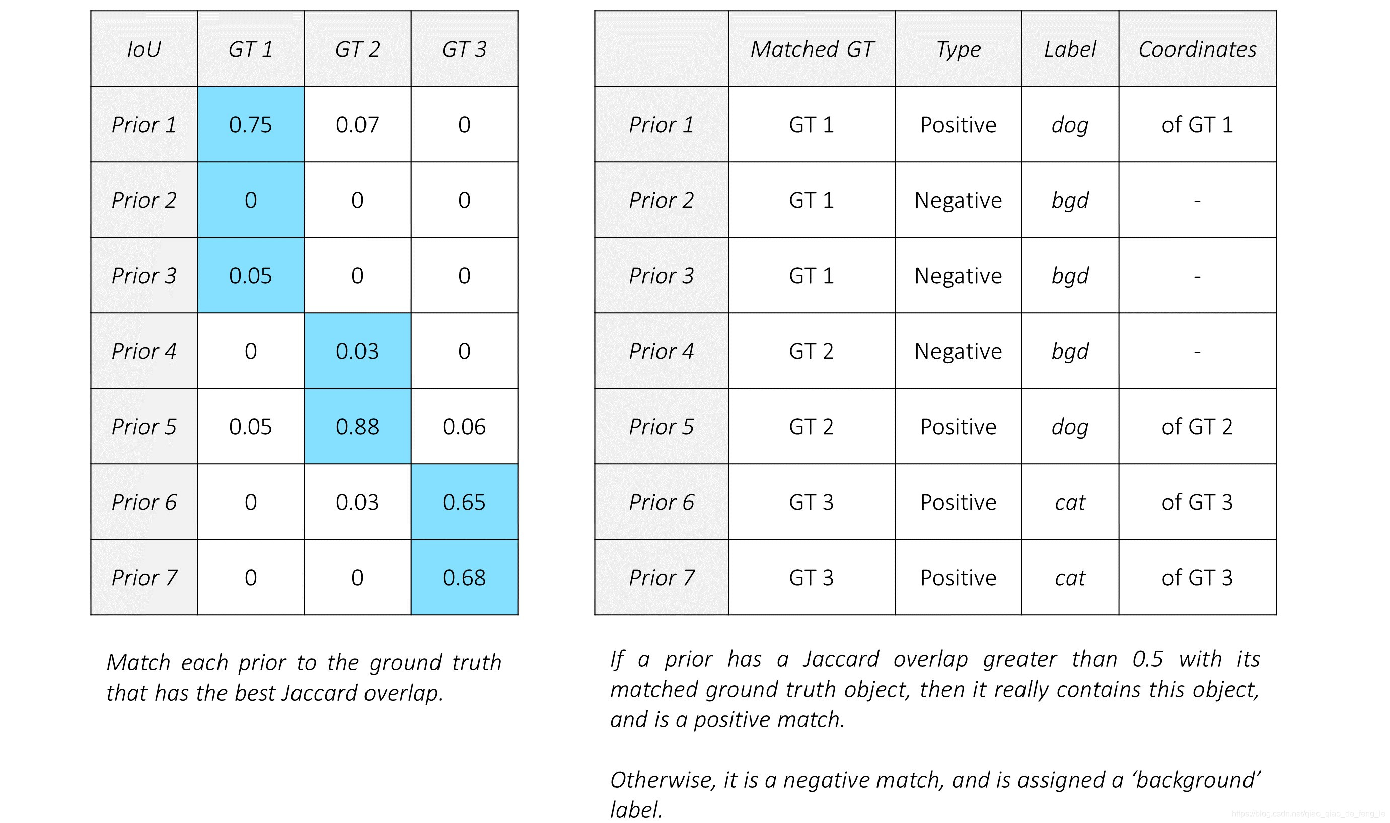
Now, each prior has a match, positive or negative. By extension, each prediction has a match, positive or negative.
Predictions that are positively matched with an object now have ground truth coordinates that will serve as targets for localization, i.e. in the regression task. Naturally, there will be no target coordinates for negative matches.
All predictions have a ground truth label, which is either the type of object if it is a positive match or a background class if it is a negative match. These are used as targets for class prediction, i.e. the classification task.
Localization loss
We have no ground truth coordinates for the negative matches. This makes perfect sense. Why train the model to draw boxes around empty space?
Therefore, the localization loss is computed only on how accurately we regress positively matched predicted boxes to the corresponding ground truth coordinates.
Since we predicted localization boxes in the form of offsets (g_c_x, g_c_y, g_w, g_h), we would also need to encode the ground truth coordinates accordingly before we calculate the loss.
The localization loss is the averaged Smooth L1 loss between the encoded offsets of positively matched localization boxes and their ground truths.

Confidence loss
Every prediction, no matter positive or negative, has a ground truth label associated with it. It is important that the model recognizes both objects and a lack of them.
However, considering that there are usually only a handful of objects in an image, the vast majority of the thousands of predictions we made do not actually contain an object. As Walter White would say, tread lightly(小心处理). If the negative matches overwhelm(淹没) the positive ones, we will end up with a model that is less likely to detect objects because, more often than not(时常), it is taught to detect the background class.
The solution may be obvious – limit the number of negative matches that will be evaluated in the loss function. But how do we choose?
Well, why not use the ones that the model was most wrong about? In other words, only use those predictions where the model found it hardest to recognize that there are no objects. This is called Hard Negative Mining.
hard negative mining解释:对于目标检测中我们会事先标记处ground truth,然后再算法中会生成一系列proposal,这些proposal有跟标记的ground truth重合的也有没重合的,那么重合度(IOU)超过一定阈值(通常0.5)的则认定为是正样本,以下的则是负样本。然后扔进网络中训练。However,这也许会出现一个问题那就是正样本的数量远远小于负样本,这样训练出来的分类器的效果总是有限的,会出现许多false positive,把其中得分较高的这些false positive当做所谓的Hard negative,既然mining出了这些Hard negative,就把这些扔进网络再训练一次,从而加强分类器判别假阳性的能力。
The number of hard negatives we will use, say N_hn, is usually a fixed multiple of the number of positive matches for this image. In this particular case, the authors have decided to use three times as many hard negatives, i.e. N_hn = 3 * N_p. The hardest negatives are discovered by finding the Cross Entropy loss for each negatively matched prediction and choosing those with top N_hn losses.
Then, the confidence loss is simply the sum of the Cross Entropy losses among the positive and hard negative matches.

You will notice that it is averaged by the number of positive matches.
Total loss
The Multibox loss is the aggregate of the two losses, combined in a ratio α.

In general, we needn’t decide on a value for α. It could be a learnable parameter.
For the SSD, however, the authors simply use α = 1, i.e. add the two losses. We’ll take it!
Processing predictions
After the model is trained, we can apply it to images. However, the predictions are still in their raw form – two tensors containing the offsets and class scores for 8732 priors. These would need to be processed to obtain final, human-interpretable(可解释的) bounding boxes with labels.
This entails(需要) the following –
-
We have 8732 predicted boxes represented as offsets (g_c_x, g_c_y, g_w, g_h) from their respective priors. Decode them to boundary coordinates, which are actually directly interpretable.
-
Then, for each non-background class,
-
Extract the scores for this class for each of the 8732 boxes.
-
Eliminate boxes that do not meet a certain threshold for this score.
-
The remaining (uneliminated) boxes are candidates for this particular class of object.
-
At this point, if you were to draw these candidate boxes on the original image, you’d see many highly overlapping boxes that are obviously redundant. This is because it’s extremely likely that, from the thousands of priors at our disposal, more than one prediction corresponds to the same object.
For instance, consider the image below.

There’s clearly only three objects in it – two dogs and a cat. But according to the model, there are three dogs and two cats.
Mind you, this is just a mild(温和的,没那么严重的) example. It could really be much, much worse.
Now, to you, it may be obvious which boxes are referring to the same object. This is because your mind can process that certain boxes coincide significantly with each other and a specific object.
In practice, how would this be done?
First, line up the candidates for each class in terms of how likely they are.

We’ve sorted them by their scores.
The next step is to find which candidates are redundant. We already have a tool at our disposal to judge how much two boxes have in common with each other – the Jaccard overlap.
So, if we were to draw up the Jaccard similarities between all the candidates in a given class, we could evaluate each pair and if found to overlap significantly, keep only the more likely candidate.

Thus, we’ve eliminated the rogue candidates – one of each animal.
This process is called Non-Maximum Suppression (NMS) because when multiple candidates are found to overlap significantly with each other such that they could be referencing the same object, we suppress all but the one with the maximum score.
Algorithmically, it is carried out as follows –
-
Upon selecting candidates for each non-background class,
-
Arrange candidates for this class in order of decreasing likelihood.
(按可能性递减的顺序安排这一类的候选人。) -
Consider the candidate with the highest score. Eliminate all candidates with lesser scores that have a Jaccard overlap of more than, say, 0.5 with this candidate.
-
Consider the next highest-scoring candidate still remaining in the pool. Eliminate all candidates with lesser scores that have a Jaccard overlap of more than 0.5 with this candidate.
-
Repeat until you run through the entire sequence of candidates.
-
The end result is that you will have just a single box – the very best one – for each object in the image.

Non-Maximum Suppression is quite crucial for obtaining quality detections.
Happily, it’s also the final step.
pytorch实现
见下篇博客。


 712
712


 被折叠的 条评论
为什么被折叠?
被折叠的 条评论
为什么被折叠?
 到【灌水乐园】发言


