


目录
记录一下数据可视化的python库matplotlib,研究并纪录一下。
matplotlib.pyplot.subplots函数。subplots可以绘制一个或多个图表。返回变量fig表示整张图片,变量ax表示图片中的各个图表,大多数情况下需要使用ax。
一、plot绘制折线图一般用法
要熟悉库的用法,多用孰能生巧。
import matplotlib
import matplotlib.pyplot as plt

x_values = range(1, 6)
y_values = [x**2 for x in x_values]

# print(plt.style.available)
# 使用seaborn绘图样式
plt.style.use('seaborn')
fig, ax = plt.subplots()
ax.plot(x_values, y_values, linewidth=3)

# xy轴的标题和图像标题
ax.set_xlabel('x values', fontsize=14)
ax.set_ylabel('y values', fontsize=14)
ax.set_title('squares', fontsize=24)

# 刻度文字的大小
ax.tick_params(axis='both', labelsize=14)

plt.show()
再试一下在同一个图表上绘制多组数据,并凸显数据之间的差别。
import csv
import matplotlib.pyplot as plt

from datetime import datetime

# filename = 'sitka_weather_07-2018_simple.csv'
filename = 'sitka_weather_2018_simple.csv'

# 读取csv数据文件
with open(filename) as f:
    reader = csv.reader(f)

    # 表头不是数据
    head_row = next(reader)

    dates, highs, lows= [], [], []
    for row in reader:
        # 第2列是日期
        cur_date = datetime.strptime(row[2], '%Y-%m-%d')

        # 第5、6列是最高气温、最低气温,注意数字的转换
        high, low = int(row[5]), int(row[6])

        dates.append(cur_date)
        highs.append(high)
        lows.append(low)

plt.style.use('seaborn')
# plt.style.use('seaborn-dark')
fig, ax = plt.subplots()

ax.plot(dates, highs, c='red')
ax.plot(dates, lows, c='blue')

# 最高、最低温度之间填充颜色凸显温差
# 入参一个x数据集,两个y数据集,指定颜色和透明度alpha
ax.fill_between(dates, highs, lows, facecolor='blue', alpha=0.2)

ax.set_xlabel('Date', fontsize=16)
ax.set_ylabel('Temperature(F)', fontsize=16)
ax.set_title('2018 Highest-Lowest Temperature')
ax.tick_params(axis='both', which='major', labelsize=16)

# plt.show()
plt.savefig('sitka_weather_2018_simple.png', bbox_inches='tight')

二、scatter绘制散点图一般用法
注意color map的用法,让数据可视化。
import matplotlib
import matplotlib.pyplot as plt
import random

x_values = range(1, 1001)
y_values = [x**2 for x in x_values]

# 使用seaborn绘图样式
plt.style.use('seaborn')
fig, ax = plt.subplots()

# 使用color map来达到随着值的改变来改变散点颜色
# 值越大颜色越深
ax.scatter(x_values, y_values, s=10, c=y_values, cmap=plt.cm.Blues,
    edgecolors='none')

# 绘制绿色起点和红色终点
ax.scatter(x_values[0], y_values[0], s=20, c='green', edgecolors='none')
ax.scatter(x_values[-1], y_values[-1], s=20, c='red', edgecolors='none')

# xy轴的标题和图像标题
ax.set_xlabel('x values', fontsize=14)
ax.set_ylabel('y values', fontsize=14)
ax.set_title('square scatter', fontsize=24)

# 刻度文字的大小
ax.tick_params(axis='both', labelsize=14, which='major')

# 刻度的范围
ax.axis([-100, 1100, -10000, 1100000])

# 显示和保存图片,bbox_inches='tight'表示去掉图片中多余的空白
# plt.show()
plt.savefig('squares_scatter.png', bbox_inches='tight')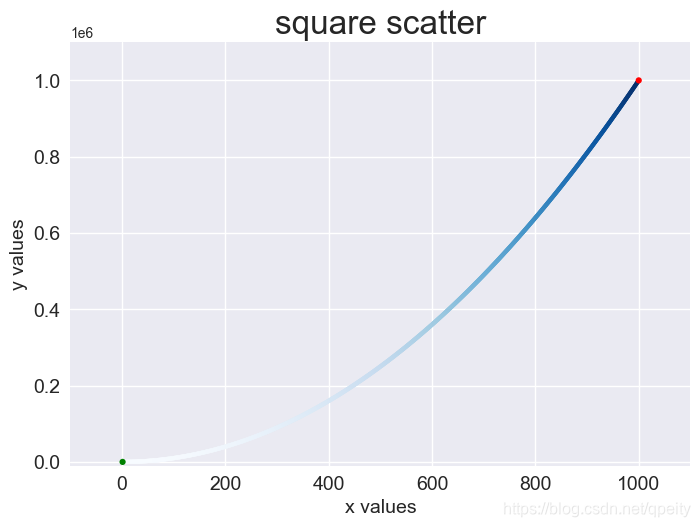
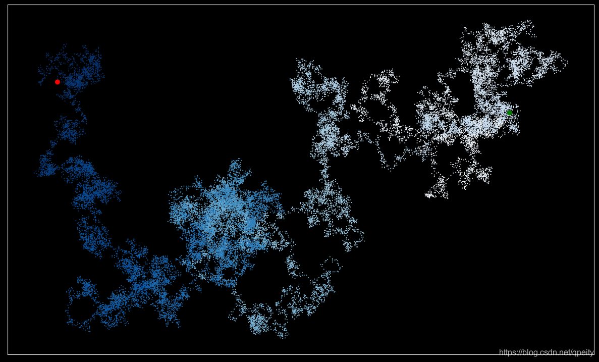
模拟一下分子的布朗运动,绿色为起点,红色为终点,模拟步数。
import matplotlib.pyplot as plt

from random import choice

class RandomWalk:
    def __init__(self, num_steps=5000, distance=5):
        # 模拟的步数
        self.num_steps = num_steps
        # 每一步最长步长
        self.distance = distance

        # 起点为(0, 0)
        self.x_values = [0]
        self.y_values = [0]

    def fill_walk(self):
        """布朗运动一下"""
        while len(self.x_values) < self.num_steps:
            x_step = self._get_setp()
            y_step = self._get_setp()
            # 不能停止不动
            if x_step == 0 and y_step == 0:
                continue

            # 更新位置
            x_step += self.x_values[-1]
            y_step += self.y_values[-1]
            self.x_values.append(x_step)
            self.y_values.append(y_step)

    def _get_setp(self):
        """随机选择方向和步长返回这一步"""
        direction = choice([-1, 1])
        distance = choice(range(0, self.distance))
        step = direction * distance
        return step

if __name__ == '__main__':
    rw = RandomWalk(num_steps=30000)
    rw.fill_walk()

    plt.style.use('dark_background')

    # 指定窗口尺寸,单位英寸
    fig, ax = plt.subplots(figsize=(15, 9))
    point_numbers = range(rw.num_steps)
    ax.scatter(rw.x_values, rw.y_values, c=point_numbers,
        cmap=plt.cm.Blues, s=2, edgecolors='none')

    # 突出起点和终点
    ax.scatter(0, 0, c='green', s=50, edgecolors='none')
    ax.scatter(rw.x_values[-1], rw.y_values[-1], c='red', s=50,
        edgecolors='none')

    # 隐藏坐标轴
    ax.get_xaxis().set_visible(False)
    ax.get_yaxis().set_visible(False)

    plt.savefig('molecular_move.png', bbox_inches='tight')


 4938
4938

 被折叠的 条评论
为什么被折叠?
被折叠的 条评论
为什么被折叠?
 到【灌水乐园】发言


