十二、机器学习算法整合（knn、朴素贝叶斯、决策树、随机森林、线性回归、岭回归、逻辑回归、聚类、支持向量机）

小树苗m

已于 2023-03-15 09:37:29 修改

阅读量2.2k

点赞数 1

分类专栏：机器学习文章标签：决策树聚类机器学习

于 2021-02-02 17:52:07 首次发布

本文链接：https://blog.csdn.net/qq_15060477/article/details/113567117

版权

机器学习专栏收录该内容

13 篇文章 1 订阅

订阅专栏

一、需要导入的库：

'''
作者:小宇
最后完成日期：2021.2.28
包含内容：knn、朴素贝叶斯、决策树、随机森林、线性回归、岭回归、逻辑回归、聚类、支持向量机
'''
from sklearn.datasets import load_breast_cancer,load_iris,load_boston,load_digits  #导入数据
from sklearn.naive_bayes import GaussianNB,MultinomialNB    #朴素贝叶斯
from sklearn.model_selection import train_test_split        #数据集划分
from sklearn.neighbors import KNeighborsClassifier          #Knn
from sklearn.tree import DecisionTreeClassifier,export_graphviz  #决策树
from sklearn.ensemble import RandomForestClassifier        #随机森林
from sklearn.linear_model import LinearRegression          #正则方程优化的线性回归
from sklearn.linear_model import Ridge                      #岭回归
from sklearn.linear_model import SGDRegressor
from sklearn.linear_model import LogisticRegression
from sklearn.cluster import KMeans
from sklearn.svm import SVC
from sklearn.feature_extraction import DictVectorizer       #特征抽取
from sklearn.model_selection import GridSearchCV            #网页搜索
from sklearn.metrics import accuracy_score              #准确率
from sklearn.metrics import classification_report
from sklearn.metrics import mean_squared_error
from sklearn.metrics import confusion_matrix
from sklearn.preprocessing import StandardScaler
import pandas as pd
import matplotlib.pyplot as plt
import numpy as np
import random

二、k近邻：

def knn_algorithm():
    '''
    knn:根据邻居进行分类，常用欧式距离，还有曼哈顿等距离计算公式
    优点：简单，易于理解和实现，无需训练
    缺点：懒惰算法，计算量大，内存开销大，必须指定K值，
         k值取小：受异常点影响
         k值取大：受样本均衡影响
    使用场景：小数据场景，几千～几万样本
    API：sklearn.neighbors.KNeighborsClassifier(n_neighbors=5,algorithm='auto')
         n_neighbors：int,可选（默认= 5），k_neighbors查询默认使用的邻居数
         algorithm：{‘auto’，‘ball_tree’，‘kd_tree’，‘brute’}，可选用于计算最近邻居的算法：
    '''
    iris = load_iris()
    x = iris.data
    y = iris.target
    x_train,x_test,y_train,y_test = train_test_split(x,y,random_state=30,train_size =0.8)
    knn = KNeighborsClassifier(n_neighbors=2,algorithm='auto')
    knn.fit(x_train,y_train)
    predictions = knn.predict(x_test)
    print(predictions)
    print(accuracy_score(y_test,predictions))
    return None

三、朴素贝叶斯：

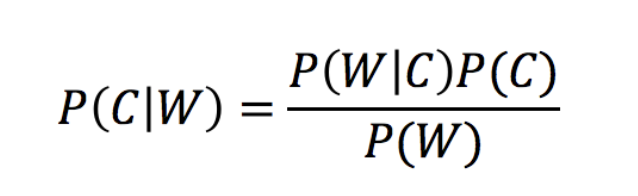
1、贝叶斯公式：
在这里插入图片描述
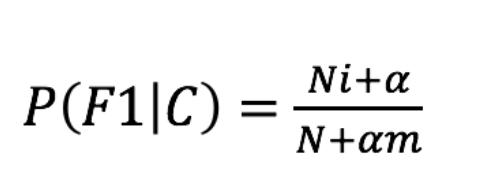
2、拉普拉斯平滑系数（防止计算出的概率为0的情况）：

def pbaye_algorithm():
    '''
    朴素贝叶斯：假定事件之间相互独立，使用贝叶斯公式对样本进行计算，常用拉普拉斯平滑系数消除由于数据集有限导致概率为0的情况；
    优点：1）有有稳定的分类效率；2）对缺失数据不太敏感，算法简单；3）分类准确度高，速度快
    缺点：特征属性有关联时其效果不好
    应用：常用语文本分类等
    API：sklearn.naive_bayes.MultinomialNB(alpha = 1.0)
         alpha：拉普拉斯平滑系数
    '''
    datal = load_breast_cancer()
    x_train,x_test,y_train,y_test = train_test_split(datal['data'],datal['target'],random_state = 20,train_size = 0.8)
    pbaye = MultinomialNB()
    pbaye.fit(x_train,y_train)
    pred = pbaye.predict(x_test)
    print(accuracy_score(y_test,pred))
    print(confusion_matrix(y_test,pred))
    print(classification_report(y_test,pred))
    return None

四、决策树

1、信息熵：
底数根据实际情况来取，此处取2

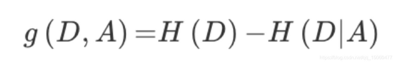
2、信息增益：
在这里插入图片描述
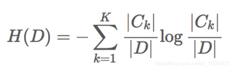
3、信息熵的计算：

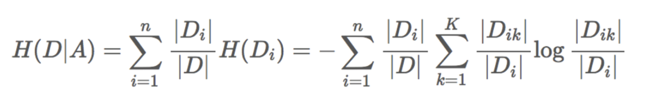
4、条件熵的计算：

def decisionc():
    '''
    决策树：1）信息熵：衡量不确定性的大小；2）条件熵H(D|A)，条件A下的信息熵；3）信息增益：不确定性减少的程度
    优点：简单，树木可视化；
    缺点：数过于复杂时，过拟合。
    改进：1）减枝cart算法；
         2）随机森林
    应用：个人信用评估等
    API：class sklearn.tree.DecisionTreeClassifier(criterion=’gini’, max_depth=None,random_state=None)
        决策树分类器
        criterion:默认’gini’系数，可选择信息增益的熵’entropy’
        max_depth:树的深度大小
        random_state:随机数种子
        max_depth:树的深度大小
    '''
    iris = datasets.load_iris()
    x_train,x_test,y_train,y_test = train_test_split(iris.data,iris.target,random_state=20,train_size=0.8)
    cls = DecisionTreeClassifier(criterion='entropy')
    cls.fit(x_train,y_train)
    pred = cls.predict(x_test)
    print(accuracy_score(y_test,pred))
    print(confusion_matrix(y_test,pred))
    print(classification_report(y_test,pred))
    #产生决策树，将得到的文本复制至：http://webgraphviz.com/可得到树
    data_l = export_graphviz(cls,out_file='tree.dot',feature_names=iris.feature_names)
    return None

五、随机森林：

def random_forest():
    '''
    随机森林：随机森林是一个包含多个决策树的分类器，并且其输出的类别是由个别树输出的类别的众数而定。
    优点：1）具有极好的准确率；2）能够有效地运行在大数据集上；3）处理具有高维特征的输入样本，无需要降维就能够评估各个特征在分类问题上的重要性。
    API：class sklearn.ensemble.RandomForestClassifier(n_estimators=10, criterion=’gini’, max_depth=None, bootstrap=True, random_state=None, min_samples_split=2)
        随机森林分类器
        n_estimators：integer，optional（default = 10）森林里的树木数量120,200,300,500,800,1200
        criteria：string，可选（default =“gini”）分割特征的测量方法
        max_depth：integer或None，可选（默认=无）树的最大深度 5,8,15,25,30
        max_features="auto”,每个决策树的最大特征数量
            If "auto", then max_features=sqrt(n_features).
            If "sqrt", then max_features=sqrt(n_features) (same as "auto").
            If "log2", then max_features=log2(n_features).
            If None, then max_features=n_features.
        bootstrap：boolean，optional（default = True）是否在构建树时使用放回抽样
        min_samples_split:节点划分最少样本数
        min_samples_leaf:叶子节点的最小样本数
    '''
    titan = pd.read_csv('titanic.csv')
    x = titan[['pclass', 'age', 'sex']]
    y = titan['survived']
    #print(x['age'])
    x['age'].fillna(x['age'].mean(), inplace=True)
    #print(x['age'])
    dict = DictVectorizer(sparse=False)
    #转化成字典并进行特征抽取
    x = dict.fit_transform(x.to_dict(orient="records"))
    x_train, x_test, y_train, y_test = train_test_split(x, y, test_size=0.3)
    rs = RandomForestClassifier()
    #下面使用网格搜索
    param = {"n_estimators": [120, 200, 300, 500, 800, 1200], "max_depth": [5, 8, 15, 25, 30]}
    rs = GridSearchCV(rs, param_grid=param, cv=3)
    rs.fit(x_train, y_train)
    pred = rs.predict(x_test)
    print(accuracy_score(y_test,pred))
    return None

六、线性回归：

def line_regression():
    '''
    线性回归：一个自变量称为单变量回归，多个自变量称为多元回归。找到最小损失，优化方法有正规方程和梯度下降两种方式
    API1（正规方程）：sklearn.linear_model.LinearRegression(fit_intercept=True)此为通过正规方程优化
            fit_intercept：是否计算偏置
            LinearRegression.coef_：回归系数
            LinearRegression.intercept_：偏置
    API2（梯度下降）：sklearn.linear_model.SGDRegressor(loss="squared_loss", fit_intercept=True, learning_rate ='invscaling', eta0=0.01)
            SGDRegressor类实现了随机梯度下降学习，它支持不同的loss函数和正则化惩罚项来拟合线性回归模型。
            loss:损失类型
            loss=”squared_loss”: 普通最小二乘法
            fit_intercept：是否计算偏置
            learning_rate : string, optional
            学习率填充
            'constant': eta = eta0
            'optimal': eta = 1.0 / (alpha * (t + t0)) [default]
            'invscaling': eta = eta0 / pow(t, power_t)
            power_t=0.25:存在父类当中
            对于一个常数值的学习率来说，可以使用learning_rate=’constant’ ，并使用eta0来指定学习率。
            SGDRegressor.coef_：回归系数
            SGDRegressor.intercept_：偏置
    '''
    data = load_boston()
    x_train, x_test, y_train, y_test = train_test_split(data.data, data.target, test_size=0.3, random_state=24)
    std_x = StandardScaler()
    x_train = std_x.fit_transform(x_train)
    x_test = std_x.transform(x_test)
    std_y = StandardScaler()
    y_train = std_y.fit_transform(y_train.reshape(-1,1))
    y_test = std_y.transform(y_test.reshape(-1,1))
    # 梯度下降进行预测
    lin = SGDRegressor()
    lin.fit(x_train, y_train)
    pre = lin.predict(x_test)
    print("权重：", lin.coef_)
    print("偏执：", lin.intercept_)
    print("预测结果:",pre)
    a = [x for x in range(len(pre))]
    plt.plot(a,pre,color = 'red')
    plt.plot(a,y_test,color = 'yellow')
    plt.show()

七、岭回归

def lin_regression():
    '''
    岭回归：一种线性回归，在回归时加上正则化限制，解决过拟合现象。有L1和L2两种正则化方法，常用L2方法。正则化力度越大，权重系数越小，正则化力度越小，权重系数越大；
    L2正则化API：sklearn.linear_model.Ridge(alpha=1.0, fit_intercept=True,solver="auto", normalize=False)
                具有l2正则化的线性回归
                alpha:正则化力度，也叫λ，λ取值：0~1 1~10
                solver:会根据数据自动选择优化方法
                sag:如果数据集、特征都比较大，选择该随机梯度下降优化
                normalize:数据是否进行标准化
                normalize=False:可以在fit之前调用preprocessing.StandardScaler标准化数据
                Ridge.coef_:回归权重
                Ridge.intercept_:回归偏置
    '''
    data = load_boston()
    x_train, x_test, y_train, y_test = train_test_split(data.data, data.target, test_size=0.3, random_state=24)
    std_x = StandardScaler()
    x_train = std_x.fit_transform(x_train)
    x_test = std_x.transform(x_test)
    std_y = StandardScaler()
    y_train = std_y.fit_transform(y_train.reshape(-1, 1))
    y_test = std_y.transform(y_test.reshape(-1, 1))
    rd = Ridge(alpha=1.0)
    rd.fit(x_train, y_train)
    print("岭回归的权重参数为：", rd.coef_)
    y_rd_predict = std_y.inverse_transform(rd.predict(x_test))
    print("岭回归的预测的结果为：", y_rd_predict)
    print("岭回归的均方误差为：", mean_squared_error(y_test, y_rd_predict))

八、逻辑回归

def logic_regression():
    '''
    逻辑回归：逻辑回归时解决二分类问题的利器，其输入为一个线性回归的结果。
    API：sklearn.linear_model.LogisticRegression(solver='liblinear', penalty=‘l2’, C = 1.0)
        solver:优化求解方式（默认开源的liblinear库实现，内部使用了坐标轴下降法来迭代优化损失函数）
        sag：根据数据集自动选择，随机平均梯度下降
        penalty：正则化的种类
        C：正则化力度
    分类评估API：sklearn.metrics.classification_report(y_true, y_pred, labels=[], target_names=None )
                y_true：真实目标值
                y_pred：估计器预测目标值
                labels:指定类别对应的数字
                target_names：目标类别名称
                return：每个类别精确率与召回率
    相关概念：精准率：召回率：准确率：
    应用：广告点击率；是否为垃圾邮件；是否患病；金融诈骗；虚假账号
    '''
    data = load_breast_cancer()
    x_train,x_test,y_train,y_test = train_test_split(data.data,data.target,random_state=30,train_size=0.8)
    lg = LogisticRegression()
    lg.fit(x_train,y_train)
    pre = lg.predict(x_test)
    print(confusion_matrix(y_test,pre))

九、聚类（k-means）:

def kmeanss():
    '''
    聚类：
    API：sklearn.cluster.KMeans(n_clusters=8,init=‘k-means++’)
        k-means聚类
        n_clusters:开始的聚类中心数量
        init:初始化方法，默认为'k-means ++’
        labels_:默认标记的类型，可以和真实值比较（不是值比较）
    轮廓系数评估API：sklearn.metrics.silhouette_score(X, labels)
                  计算所有样本的平均轮廓系数
                  X：特征值
                  labels：被聚类标记的目标值
    '''
    x1 = np.array([1, 2, 3, 1, 5, 6, 5, 5, 6, 7, 8, 9, 9])
    x2 = np.array([1, 3, 2, 2, 8, 6, 7, 6, 7, 1, 2, 1, 3])
    # x = np.array(list(zip(x1,x2)).reshape(len(x1),2))
    x = np.array(list(zip(x1, x2)))
    plt.figure(figsize=(10, 10))
    plt.xlim([0, 10])
    plt.ylim([0, 10])
    plt.title('sample')
    plt.scatter(x1, x2)
    plt.show()
    kmeans_model = KMeans(n_clusters=3).fit(x)
    colors = ['b', 'g', 'r']
    markers = ['o', '^', '+']
    for i, j in enumerate(kmeans_model.labels_):
        plt.plot(x[i], x2[i], colors=colors[j], markers=markers[j], ls='None')
    plt.xlim([0, 10])
    plt.ylim([0, 10])
    plt.show()
    print(x)

十、支持向量机（svm）：

def svmm():
    '''
    支持向量机(完善)：用超平面对高纬空间中的样本进行分类，为了解决线性不可分问题，引入了核函数，常用核函数有线性核函数、多项式核函数、高斯核函数和sigmoid核函数
    API:sklearn.svm.SVC(C=1.0, kernel='rbf', degree=3, gamma='auto', coef0=0.0, shrinking=True,
                probability=False, tol=0.001, cache_size=200, class_weight=None,
                verbose=False, max_iter=-1, decision_function_shape='ovr',
                random_state=None)
                C （float参数 默认值为1.0）:惩罚项系数
                kernel （str参数 默认为‘rbf’）：核函数选择（linear：线性核函数，poly：多项式核函数，rbf：径像核函数/高斯核，sigmod：sigmod核函数，precomputed：核矩阵）
                degree （int型参数 默认为3）：只对'kernel=poly'(多项式核函数)有用，是指多项式核函数的阶数n，如果给的核函数参数是其他核函数，则会自动忽略该参数。
                gamma （float参数 默认为auto）：如果gamma设置为auto，代表其值为样本特征数的倒数，即1/n_features，也有其他值可设定。
                coef0:（float参数 默认为0.0）：核函数中的独立项，只有对‘poly’和‘sigmod’核函数有用，是指其中的参数c。
                probability（ bool参数 默认为False）：是否启用概率估计。
                shrinkintol: float参数 默认为1e^-3g（bool参数 默认为True）：表示是否选用启发式收缩方式。
                tol（ float参数 默认为1e^-3）：svm停止训练的误差精度，也即阈值。
                cache_size（float参数 默认为200）：指定训练所需要的内存，以MB为单位。
                class_weight（字典类型或者‘balance’字符串。默认为None）：该参数表示给每个类别分别设置不同的惩罚参数C，如果没有给，则会给所有类别都给C=1，即前面参数指出的参数C。如果给定参数‘balance’，则使用y的值自动调整与输入数据中的类频率成反比的权重。
                verbose （ bool参数 默认为False）：是否启用详细输出。
                max_iter （int参数 默认为-1）：最大迭代次数，-1表示不受限制。
                random_state（int，RandomState instance ，None 默认为None）：随机数种子
    '''
    daj = load_digits()
    images = daj.images
    labels = daj.target
    n_samples = len(images)
    image_vectors = images.reshape((n_samples,-1))
    sample_index = list(range(n_samples))
    test_size = int(n_samples*2)
    random.shuffle(sample_index)
    train_index,test_index = sample_index[test_size:],sample_index[:test_size]
    x_train,y_train = image_vectors[train_index],labels[train_index]
    x_test, y_test = image_vectors[test_index], labels[test_index]
    classifier = SVC(kernel='rbf',C=1.0,gamma=0.001)
    classifier.fit(x_train,y_train)
    pre = classifier.predict(x_test)
    print(classification_report(y_test,pre))
    print(confusion_matrix(y_test,pre))

小树苗m

关注

1
点赞
踩
38

收藏

觉得还不错? 一键收藏
打赏
0
评论
十二、机器学习算法整合（knn、朴素贝叶斯、决策树、随机森林、线性回归、岭回归、逻辑回归、聚类、支持向量机）

一、需要导入的库：'''作者:小宇最后完成日期：2021.2.28包含内容：支持向量机、AdaBoost、朴素贝叶斯、Knn、决策树、随机森林、线性回归'''from sklearn.datasets import load_breast_cancer,load_iris,load_boston,load_digits #导入数据from sklearn.naive_bayes import GaussianNB,MultinomialNB #朴素贝叶斯from sklearn.mo
复制链接

扫一扫