


练习一:线性回归
目录
1.包含的文件
2.单元线性回归
3.多元线性回归
1.包含的文件

| 文件名 | 含义 |
| ex1.py | 单元线性回归 |
| ex1_multi.py | 多元线性回归 |
| ex1data1.txt | 单变量线性回归数据集 |
| ex1data2.txt | 多变量线性回归数据集 |
| plotData.py | 数据可视化 |
| computeCost.py | 损失函数 |
| gradientDescent.py | 梯度下降 |
| featureNormalize.py | 特征归一化 |
| normalEqn.py | 正规方程求解线性回归程序 |
红色部分需要自己填写。
2.单元线性回归
项目需要的包
import matplotlib.pyplot as plt
import numpy as np
from matplotlib.colors import LogNorm
from mpl_toolkits.mplot3d import axes3d, Axes3D
from computeCost import *
from gradientDescent import *
from plotData import *
import matplotlib.pyplot as plt
2.1可视化数据集
- 主程序
# ===================== Part 1: Plotting =====================
print('Plotting Data...')


data = np.loadtxt('ex1data1.txt', delimiter=',', usecols=(0, 1))
X = data[:, 0]
y = data[:, 1]
m = y.size


plot_data(X, y)

input('Program paused. Press ENTER to continue')
- 可视化函数plotData.py
import matplotlib.pyplot as plt


def plot_data(x, y):
    # ===================== Your Code Here =====================
    # Instructions : Plot the training data into a figure using the matplotlib.pyplot
    #                using the "plt.scatter" function. Set the axis labels using
    #                "plt.xlabel" and "plt.ylabel". Assume the population and revenue data
    #                have been passed in as the x and y.

    # Hint : You can use the 'marker' parameter in the "plt.scatter" function to change the marker type (e.g. "x", "o").
    #        Furthermore, you can change the color of markers with 'c' parameter.
    plt.scatter(x,y,marker='o',s=50,cmap='Blues',alpha=0.3)  #绘制散点图
    plt.xlabel('population')  #设置x轴标题
    plt.ylabel('profits')   #设置y轴标题

    # ===========================================================

plt.show()- 运行结果:

2.2梯度下降
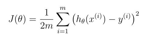
- 单变量线性回归的目标是使损失函数最小化:
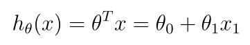
- 单变量线性模型是:
- 编写计算线性回归代价函数的程序computeCost.py
import numpy as np


def compute_cost(X, y, theta):
    # Initialize some useful values
    m = y.size
    cost = 0

    # ===================== Your Code Here =====================
    # Instructions : Compute the cost of a particular choice of theta.
    #                You should set the variable "cost" to the correct value.
    h_out = theta*X#回归输出
    error = (h_out.sum(axis=1)-y)*(h_out.sum(axis=1)-y)#先按行求和  再与Y按列求差 再内积
    error_all = error.sum(axis=0)#按列求和 得到总误差
    cost = 1/(2*m)*error_all

    # ==========================================================

    return cost
- 运行结果为:
Initial cost : 32.0727338775 (This value should be about 32.07)
- 梯度下降为:

- 编写梯度下降程序gradientDescent.py
import numpy as np
from computeCost import *


def gradient_descent(X, y, theta, alpha, num_iters):
    # Initialize some useful values
    m = y.size
    J_history = np.zeros(num_iters)

    for i in range(0, num_iters):
        # ===================== Your Code Here =====================
        # Instructions : Perform a single gradient step on the parameter vector theta
        #
        # Hint: X.shape = (97, 2), y.shape = (97, ), theta.shape = (2, )
        h_out = theta * X#回归输出
        error = h_out.sum(axis=1) - y#先按行求和 a1x1+a0 再与y求偏差
        error_2d =  error.reshape(m,1)#转换成2维数组进行乘法
        error_all = error_2d*X#是一个 m*2大小的数组
        theta = theta -  alpha*(1/m)*error_all.sum(axis = 0)#按列求和成 1*2大小数组更新
        # ===========================================================
        # Save the cost every iteration
        J_history[i] = compute_cost(X, y, theta)

return theta, J_history- 运行结果为:
Theta found by gradient descent: [-3.63029144 1.16636235]
- 主程序
# ===================== Part 2: Gradient descent =====================
print('Running Gradient Descent...')
X = np.c_[np.ones(m), X]  # Add a column of ones to X
theta = np.zeros(2)  # initialize fitting parameters

# Some gradient descent settings
iterations = 1500
alpha = 0.01
# Compute and display initial cost
print('Initial cost : ' + str(compute_cost(X, y, theta)) + ' (This value should be about 32.07)')
theta, J_history = gradient_descent(X, y, theta, alpha, iterations)
print('Theta found by gradient descent: ' + str(theta.reshape(2)))

# Plot the linear fit
plt.figure(0)
line1, = plt.plot(X[:, 1], np.dot(X, theta), label='Linear Regression')
plt.legend(handles=[line1])
input('Program paused. Press ENTER to continue')

# Predict values for population sizes of 35,000 and 70,000
predict1 = np.dot(np.array([1, 3.5]), theta)
print('For population = 35,000, we predict a profit of {:0.3f} (This value should be about 4519.77)'.format(predict1*10000))
predict2 = np.dot(np.array([1, 7]), theta)
print('For population = 70,000, we predict a profit of {:0.3f} (This value should be about 45342.45)'.format(predict2*10000))

input('Program paused. Press ENTER to continue')- 利用训练好的参数进行预测,与期望值进行比较,验证我们的程序是正确的:
For population = 35,000, we predict a profit of 4519.768 (This value should be about 4519.77)
For population = 70,000, we predict a profit of 45342.450 (This value should be about 45342.45)
- 拟合的直线:

2.3可视化代价函数
# ===================== Part 3: Visualizing J(theta0, theta1) =====================
print('Visualizing J(theta0, theta1) ...')

theta0_vals = np.linspace(-10, 10, 100)  #参数1的取值
theta1_vals = np.linspace(-1, 4, 100)    #参数2的取值

xs, ys = np.meshgrid(theta0_vals, theta1_vals)   #生成网格
J_vals = np.zeros(xs.shape)


for i in range(0, theta0_vals.size):
    for j in range(0, theta1_vals.size):
        t = np.array([theta0_vals[i], theta1_vals[j]])
        J_vals[i][j] = compute_cost(X, y, t)    #计算每个网格点的代价函数值

J_vals = np.transpose(J_vals)

fig1 = plt.figure(1)      #绘制3d图形
ax = fig1.gca(projection='3d')
ax.plot_surface(xs, ys, J_vals)
plt.xlabel(r'$\theta_0$')
plt.ylabel(r'$\theta_1$')

#绘制等高线图 相当于3d图形的投影
plt.figure(2)
lvls = np.logspace(-2, 3, 20)
plt.contour(xs, ys, J_vals, levels=lvls, norm=LogNorm())
plt.plot(theta[0], theta[1], c='r', marker="x")
- 可视化效果


3.多元线性回归
3.1特征归一化
- 编写归一化代码featureNormalize.py
import numpy as np


def feature_normalize(X):
    # You need to set these values correctly
    n = X.shape[1]  # the number of features
    X_norm = X
    mu = np.zeros(n)
    sigma = np.zeros(n)

    # ===================== Your Code Here =====================
    # Instructions : First, for each feature dimension, compute the mean
    #                of the feature and subtract it from the dataset,
    #                storing the mean value in mu. Next, compute the
    #                standard deviation of each feature and divide
    #                each feature by its standard deviation, storing
    #                the standard deviation in sigma
    #
    #                Note that X is a 2D array where each column is a
    #                feature and each row is an example. You need
    #                to perform the normalization separately for
    #                each feature.
    #
    # Hint: You might find the 'np.mean' and 'np.std' functions useful.
    #       To get the same result as Octave 'std', use np.std(X, 0, ddof=1)
    #
    mu = np.mean(X_norm,axis=0)#按列求平均值
    sigma = np.std(X_norm, axis=0) # axis=0计算每一列的标准差
    X_norm = (X-mu)/sigma

    # ===========================================================

    return X_norm, mu, sigma
- 测试函数:
# ===================== Part 1: Feature Normalization =====================
print('Loading Data...')
data = np.loadtxt('ex1data2.txt', delimiter=',', dtype=np.int64)
X = data[:, 0:2]
y = data[:, 2]
m = y.size

# Print out some data points
print('First 10 examples from the dataset: ')
for i in range(0, 10):
    print('x = {}, y = {}'.format(X[i], y[i]))

input('Program paused. Press ENTER to continue')

# Scale features and set them to zero mean
print('Normalizing Features ...')

X, mu, sigma = feature_normalize(X)
X = np.c_[np.ones(m), X]  # Add a column of ones to X
3.2梯度下降
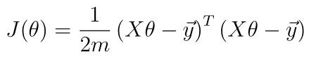
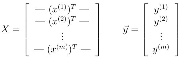
- 多元线性回归,要以向量的形式:
- 编写多元参数梯度下降程序gradientDescent.py
def gradient_descent_multi(X, y, theta, alpha, num_iters):
    # Initialize some useful values
    m = y.size
    J_history = np.zeros(num_iters)

    for i in range(0, num_iters):
        # ===================== Your Code Here =====================
        # Instructions : Perform a single gradient step on the parameter vector theta
        #
        h_out = theta * X#回归输出
        error = h_out.sum(axis=1) - y#先按行求和 a1x1+a0 再与y求偏差
        error_2d =  error.reshape(m,1)#转换成2维数组进行乘法
        error_all = error_2d*X#是一个 m*2大小的数组
        theta = theta -  alpha*(1/m)*error_all.sum(axis = 0)#按列求和成 1*2大小数组更新

        # ===========================================================
        # Save the cost every iteration
        J_history[i] = compute_cost(X, y, theta)

return theta, J_history- 测试代码:
# ===================== Part 2: Gradient Descent =====================

# ===================== Your Code Here =====================
# Instructions : We have provided you with the following starter
#                code that runs gradient descent with a particular
#                learning rate (alpha).
#
#                Your task is to first make sure that your functions -
#                computeCost and gradientDescent already work with
#                this starter code and support multiple variables.
#
#                After that, try running gradient descent with
#                different values of alpha and see which one gives
#                you the best result.
#
#                Finally, you should complete the code at the end
#                to predict the price of a 1650 sq-ft, 3 br house.
#
# Hint: At prediction, make sure you do the same feature normalization.
#

print('Running gradient descent ...')

# Choose some alpha value
alpha = 0.03

num_iters = 500

# Init theta and Run Gradient Descent
theta = np.zeros(3)
theta, J_history = gradient_descent_multi(X, y, theta, alpha, num_iters)

# Plot the convergence graph
plt.figure()
plt.plot(np.arange(J_history.size), J_history)
plt.xlabel('Number of iterations')
plt.ylabel('Cost J')

# Display gradient descent's result
print('Theta computed from gradient descent : \n{}'.format(theta))

# Estimate the price of a 1650 sq-ft, 3 br house
# ===================== Your Code Here =====================
# Recall that the first column of X is all-ones. Thus, it does
# not need to be normalized.
a1 = np.array([1650, 3])
a1_nromal = (a1 - mu)/sigma
X1 = np.c_[np.ones(1), a1_nromal.reshape(1,2)]#扩充一列
price = (theta*X1).sum(axis=1)[0] # You should change this


# ==========================================================

print('Predicted price of a 1650 sq-ft, 3 br house (using gradient descent) : {:0.3f}'.format(price))

input('Program paused. Press ENTER to continue')- 梯度下降法求解的最优参数,样例的预测价格以及代价函数随迭代次数的变化曲线

3.3正规方程直接求解
- 正规方程:
![]()
- 编写代码normalEqn.py:
import numpy as np

def normal_eqn(X, y):
    theta = np.zeros((X.shape[1], 1))

    # ===================== Your Code Here =====================
    # Instructions : Complete the code to compute the closed form solution
    #                to linear regression and put the result in theta
    #
    X_mat = np.mat(X)
    y_mat = np.mat(y)
    A = np.dot(X_mat.T, X_mat)
    B = np.dot(A.I,X.T)
    theta = np.dot(B,y)
    #theta = np.dot(np.dot(np.dot(X_mat.T, X_mat).I,X_mat.T), y).T#这样写是错误的
    theta = theta.getA()#矩阵转换成数组
    return theta
- 测试程序:
# ===================== Part 3: Normal Equations =====================

print('Solving with normal equations ...')

# ===================== Your Code Here =====================
# Instructions : The following code computes the closed form
#                solution for linear regression using the normal
#                equations. You should complete the code in
#                normalEqn.py
#
#                After doing so, you should complete this code
#                to predict the price of a 1650 sq-ft, 3 br house.
#

# Load data
data = np.loadtxt('ex1data2.txt', delimiter=',', dtype=np.int64)
X = data[:, 0:2]
y = data[:, 2]
m = y.size

# Add intercept term to X
X = np.c_[np.ones(m), X]

theta = normal_eqn(X, y)

# Display normal equation's result
print('Theta computed from the normal equations : \n{}'.format(theta))

# Estimate the price of a 1650 sq-ft, 3 br house
# ===================== Your Code Here =====================
a2 = np.array([1650, 3])
X2 = np.c_[np.ones(1), a2.reshape(1,2)]#扩充一列
price = (theta*X2).sum(axis=1)[0]  # You should change this


# ==========================================================

print('Predicted price of a 1650 sq-ft, 3 br house (using normal equations) : {:0.3f}'.format(price))

input('ex1_multi Finished. Press ENTER to exit')
注:所有代码及说明PDF在全部更新完后统一上传。


 2万+
2万+


 被折叠的 条评论
为什么被折叠?
被折叠的 条评论
为什么被折叠?
 到【灌水乐园】发言


