吴恩达cs229|编程作业第五周（Python）

最新推荐文章于 2023-03-21 20:24:36 发布

NotFound1911

最新推荐文章于 2023-03-21 20:24:36 发布

阅读量1.1k

点赞数

分类专栏：自学

本文链接：https://blog.csdn.net/qq_24739717/article/details/88749596

版权

自学专栏收录该内容

78 篇文章 17 订阅

订阅专栏

练习五：正则化线性回归与偏置vs方差

1.包含的文件。

2.正则化线性回归。

3.偏差和方差。

4.多项式回归。

1.包含的文件

文件名	含义
ex5.py	实验主程序
ex5data1.mat	数据集
featureNormalize.py	特征缩放程序
trainLinearReg.py	训练程序
plotFit.py	绘制拟合曲线
learningCurve.py	绘制学习曲线程序
linearRegCostFunction.py	线性回归(正则化）代价函数
ployFeatures.py	给原始特征增加特征
validationCurve.py	验证曲线程序

红色部分需要自己填写。

2.正则化线性回归。

加载需要的包和初始化：

import matplotlib.pyplot as plt
import numpy as np
import scipy.io as scio
import linearRegCostFunction as lrcf
import trainLinearReg as tlr
import learningCurve as lc
import polyFeatures as pf
import featureNormalize as fn
import plotFit as plotft
import validationCurve as vc

plt.ion()
np.set_printoptions(formatter={'float': '{: 0.6f}'.format})

2.1数据可视化

测试代码：

# ===================== Part 1: Loading and Visualizing Data =====================
# We start the exercise by first loading and visualizing the dataset.
# The following code will load the dataset into your environment and pot
# the data.
#

# Load Training data
print('Loading and Visualizing data ...')

# Load from ex5data1:
data = scio.loadmat('ex5data1.mat')
X = data['X']
y = data['y'].flatten()
Xval = data['Xval']
yval = data['yval'].flatten()
Xtest = data['Xtest']
ytest = data['ytest'].flatten()

m = y.size

# Plot training data
plt.figure()
plt.scatter(X, y, c='r', marker="x")
plt.xlabel('Change in water level (x)')
plt.ylabel('Water folowing out of the dam (y)')

input('Program paused. Press ENTER to continue')

测试结果：

2.2正则化线性回归代价函数和梯度

代价函数：

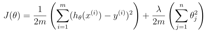
正则化线性回归梯度：

编写linearRegCostFunction.py：

import numpy as np


def linear_reg_cost_function(theta, x, y, lmd):
    # Initialize some useful values
    m = y.size

    # You need to return the following variables correctly
    cost = 0
    grad = np.zeros(theta.shape)

    # ===================== Your Code Here =====================
    # Instructions : Compute the cost and gradient of regularized linear
    #                regression for a particular choice of theta
    #
    #                You should set 'cost' to the cost and 'grad'
    #                to the gradient
    #
    
    h_out= np.dot(x,theta)#使用点乘 生成一维的数组  
    theta_lmd = theta[1:]#第一个theta不正则化
    error = h_out- y# 线性回归输出h 再与y求偏差
    error_2d =  error.reshape(m,1)#转换成2维数组进行乘法
    error_all = error_2d*x#是一个 m*n大小的数组
    
    cost = np.mean(error*error,axis=0)*(1/2)\
     +lmd/(2*m)*(theta_lmd*theta_lmd).sum()
 
    #j>=1加上正则化项 j=0不加
    grad[0] = (1/m)*error_all[:,0].sum(axis=0)
    grad[1:] = (1/m)*error_all[:,1:].sum(axis=0)+lmd/m*theta_lmd

    # ==========================================================

    return cost, grad

测试代码：

# ===================== Part 2: Regularized Linear Regression Cost =====================
# You should now implement the cost function for regularized linear regression
#

theta = np.ones(2)
cost, _ = lrcf.linear_reg_cost_function(theta, np.c_[np.ones(m), X], y, 1)

print('Cost at theta = [1  1]: {:0.6f}\n(this value should be about 303.993192'.format(cost))

input('Program paused. Press ENTER to continue')

# ===================== Part 3: Regularized Linear Regression Gradient =====================
# You should now implement the gradient for regularized linear regression
#

theta = np.ones(2)
cost, grad = lrcf.linear_reg_cost_function(theta, np.c_[np.ones(m), X], y, 1)

print('Gradient at theta = [1  1]: {}\n(this value should be about [-15.303016  598.250744]'.format(grad))

input('Program paused. Press ENTER to continue')

测试结果：

Program paused. Press ENTER to continue
Cost at theta = [1 1]: 303.993192
(this value should be about 303.993192

Program paused. Press ENTER to continue
Gradient at theta = [1 1]: [-15.303016 598.250744]
(this value should be about [-15.303016 598.250744]

2.3拟合线性回归

拟合参数训练线性回归trainLinearReg.py：

import numpy as np
import linearRegCostFunction as lrcf
import scipy.optimize as opt


def train_linear_reg(x, y, lmd):
    initial_theta = np.ones(x.shape[1])

    def cost_func(t):
        return lrcf.linear_reg_cost_function(t, x, y, lmd)[0]

    def grad_func(t):
        return lrcf.linear_reg_cost_function(t, x, y, lmd)[1]
    #调用高级优化方法
    theta, *unused = opt.fmin_cg(cost_func, initial_theta, grad_func, maxiter=200, disp=False,
                                     full_output=True)

    return theta

测试代码：


# ===================== Part 4: Train Linear Regression =====================
# Once you have implemented the cost and gradient correctly, the
# train_linear_reg function will use your cost function to train regularzized linear regression.
#
# Write Up Note : The data is non-linear, so this will not give a great fit.
#

# Train linear regression with lambda = 0
lmd = 0

theta = tlr.train_linear_reg(np.c_[np.ones(m), X], y, lmd)

# Plot fit over the data
plt.plot(X, np.dot(np.c_[np.ones(m), X], theta))

input('Program paused. Press ENTER to continue')

测试结果：

3.偏差和方差

线性回归学习曲线：

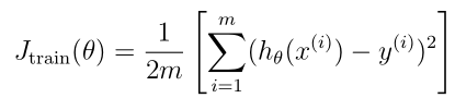
编写绘制曲线learningCurve.py：

import numpy as np
import trainLinearReg as tlr
import linearRegCostFunction as lrcf


def learning_curve(X, y, Xval, yval, lmd):
    # Number of training examples
    m = X.shape[0]

    # You need to return these values correctly
    error_train = np.zeros(m)
    error_val = np.zeros(m)

    # ===================== Your Code Here =====================
    # Instructions : Fill in this function to return training errors in
    #                error_train and the cross validation errors in error_val.
    #                i.e., error_train[i] and error_val[i] should give you
    #                the errors obtained after training on i examples
    #
    # Note : You should evaluate the training error on the first i training
    #        examples (i.e. X[:i] and y[:i])
    #
    #        For the cross-validation error, you should instead evaluate on
    #        the _entire_ cross validation set (Xval and yval).
    #
    # Note : If you're using your cost function (linear_reg_cost_function)
    #        to compute the training and cross validation error, you should
    #        call the function with the lamdba argument set to 0.
    #        Do note that you will still need to use lamdba when running the
    #        training to obtain the theta parameters.
    #
    #从0开始逐渐增加训练样本个数
    for i in range(m):
        x_i = X[:i+1]
        y_i = y[:i+1]
        #线性回归求得 theta
        theta = tlr.train_linear_reg(x_i, y_i, lmd)
        #theta 分别用于训练集 和 验证集  求得线性回归误差
        error_train[i] = lrcf.linear_reg_cost_function(theta, x_i, y_i, 0)[0]
        error_val[i] = lrcf.linear_reg_cost_function(theta, Xval, yval, 0)[0]

    # ==========================================================

    return error_train, error_val

测试代码：

# ===================== Part 5: Learning Curve for Linear Regression =====================
# Next, you should implement the learning_curve function.
#
# Write up note : Since the model is underfitting the data, we expect to
#                 see a graph with "high bias" -- Figure 3 in ex5.pdf
#

lmd = 0
error_train, error_val = lc.learning_curve(np.c_[np.ones(m), X], y, np.c_[np.ones(Xval.shape[0]), Xval], yval, lmd)

plt.figure()
plt.plot(np.arange(m), error_train, np.arange(m), error_val)
plt.title('Learning Curve for Linear Regression')
plt.legend(['Train', 'Cross Validation'])
plt.xlabel('Number of Training Examples')
plt.ylabel('Error')
plt.axis([0, 13, 0, 150])

input('Program paused. Press ENTER to continue')

测试结果：

曲线特点：验证误差随样本增加不断减小，并趋于平缓；训练误差随样本增加不断增大，最后也趋于平缓；并且二者非常接近，交界处对应的误差比较大。根据学习曲线的特点，此时模型出现了高偏差的情况，也就是欠拟合。此时增加更多的训练样本用处不大，应该增加更多的输入特征。

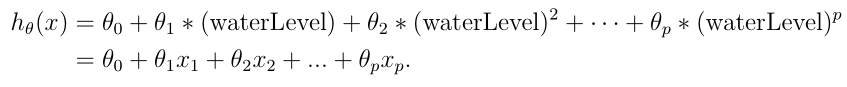
4.多项式回归

对于多项式回归，我们的假设有这种形式（增加数据特征数量）：

查看特征缩放程序featureNormalize.py

import numpy as np


def feature_normalize(X):
    mu = np.mean(X, 0)  #求特征矩阵每一列的均值
    sigma = np.std(X, 0, ddof=1)#求特征矩阵每一列的标准差
    X_norm = (X - mu) / sigma  #对特征矩阵每一列进行缩放
 
    return X_norm, mu, sigma

编写特征映射程序ployFeatures.py：

import numpy as np


def poly_features(X, p):
    # You need to return the following variable correctly.
    X_poly = np.zeros((X.size, p))

    # ===================== Your Code Here =====================
    # Instructions : Given a vector X, return a matrix X_poly where the p-th
    #                column of X contains the values of X to the p-th power.
    #
    for i in range(p):
        if i == 0:
            X_add = X
        else :
            X_add = X_add*X
        X_poly[:,i] = X_add.flatten()
    # ==========================================================

    return X_poly

测试代码（增加特征和训练拟合线性回归）：

# ===================== Part 6 : Feature Mapping for Polynomial Regression =====================
# One solution to this is to use polynomial regression. You should now
# complete polyFeatures to map each example into its powers
#

p = 5

# Map X onto Polynomial Features and Normalize
X_poly = pf.poly_features(X, p)
X_poly, mu, sigma = fn.feature_normalize(X_poly)
X_poly = np.c_[np.ones(m), X_poly]

# Map X_poly_test and normalize (using mu and sigma)
X_poly_test = pf.poly_features(Xtest, p)
X_poly_test -= mu
X_poly_test /= sigma
X_poly_test = np.c_[np.ones(X_poly_test.shape[0]), X_poly_test]

# Map X_poly_val and normalize (using mu and sigma)
X_poly_val = pf.poly_features(Xval, p)
X_poly_val -= mu
X_poly_val /= sigma
X_poly_val = np.c_[np.ones(X_poly_val.shape[0]), X_poly_val]

print('Normalized Training Example 1 : \n{}'.format(X_poly[0]))

input('Program paused. Press ENTER to continue')

# ===================== Part 7 : Learning Curve for Polynomial Regression =====================
# Now, you will get to experiment with polynomial regression with multiple
# values of lambda. The code below runs polynomial regression with
# lambda = 0. You should try running the code with different values of
# lambda to see how the fit and learning curve change.
#

lmd = 1
theta = tlr.train_linear_reg(X_poly, y, lmd)

# Plot trainint data and fit
plt.figure()
plt.scatter(X, y, c='r', marker="x")
plotft.plot_fit(np.min(X), np.max(X), mu, sigma, theta, p)
plt.xlabel('Change in water level (x)')
plt.ylabel('Water folowing out of the dam (y)')
plt.ylim([0, 60])
plt.title('Polynomial Regression Fit (lambda = {})'.format(lmd))

error_train, error_val = lc.learning_curve(X_poly, y, X_poly_val, yval, lmd)
plt.figure()
plt.plot(np.arange(m), error_train, np.arange(m), error_val)
plt.title('Polynomial Regression Learning Curve (lambda = {})'.format(lmd))
plt.legend(['Train', 'Cross Validation'])
plt.xlabel('Number of Training Examples')
plt.ylabel('Error')
plt.axis([0, 13, 0, 150])

print('Polynomial Regression (lambda = {})'.format(lmd))
print('# Training Examples\tTrain Error\t\tCross Validation Error')
for i in range(m):
    print('  \t{}\t\t{}\t{}'.format(i, error_train[i], error_val[i]))

input('Program paused. Press ENTER to continue')

测试结果：

Normalized Training Example 1 :
[ 1.000000 -0.362141 -0.755087 0.182226 -0.706190 0.306618]

Program paused. Press ENTER to continue
Polynomial Regression (lambda = 1)
# Training Examples Train Error Cross Validation Error
0 3.559734834809816e-29 138.84677697582416
1 0.046813414357849865 143.06103979015688
2 3.30878030050552 7.257068884003384
3 1.7528614019177517 6.988497062932704
4 1.4958586625205554 3.779076540658268
5 1.109639194523331 4.792229457483858
6 1.55943376402576 3.7789767443457443
7 1.3627902650800985 3.7813696626421724
8 1.4801169453728649 4.277962524659826
9 1.3696114992729276 4.137274998453949
10 1.2419827237205616 4.187257261122695
11 1.937233763118866 3.7368928407747473

增加多项式特征后，验证误差随训练样本的增加先不断减小，到达一个最优值后，又开始上升；

而训练误差一直都非常小，接近0。不难判断此时出现了过拟合的情况，可以进行正则化，调整一下lambda的值。

模型选择，通过验证集选择一个最优的lambda值，编写validationCurve.py：

import numpy as np
import trainLinearReg as tlr
import linearRegCostFunction as lrcf


def validation_curve(X, y, Xval, yval):
    # Selected values of lambda (don't change this)
    lambda_vec = np.array([0., 0.001, 0.003, 0.01, 0.03, 0.1, 0.3, 1, 3, 10])

    # You need to return these variables correctly.
    error_train = np.zeros(lambda_vec.size)
    error_val = np.zeros(lambda_vec.size)

    # ===================== Your Code Here =====================
    # Instructions : Fill in this function to return training errors in
    #                error_train and the validation errors in error_val. The
    #                vector lambda_vec contains the different lambda parameters
    #                to use for each calculation of the errors, i.e,
    #                error_train[i], and error_val[i] should give
    #                you the errors obtained after training with
    #                lmd = lambda_vec[i]
    #
    # 遍历lmd的值
    i = 0
    for lmd in lambda_vec:
        #线性回归求得 theta
        theta = tlr.train_linear_reg(X, y, lmd)
        #theta 分别用于训练集 和 验证集  求得线性回归误差
        error_train[i] = lrcf.linear_reg_cost_function(theta, X, y, 0)[0]
        error_val[i] = lrcf.linear_reg_cost_function(theta, Xval, yval, 0)[0]
        i = i+1
    # ==========================================================

    return lambda_vec, error_train, error_val

测试代码：

# ===================== Part 8 : Validation for Selecting Lambda =====================
# You will now implement validationCurve to test various values of
# lambda on a validation set. You will then use this to select the
# 'best' lambda value.

lambda_vec, error_train, error_val = vc.validation_curve(X_poly, y, X_poly_val, yval)

plt.figure()
plt.plot(lambda_vec, error_train, lambda_vec, error_val)
plt.legend(['Train', 'Cross Validation'])
plt.xlabel('lambda')
plt.ylabel('Error')

input('ex5 Finished. Press ENTER to exit')

测试结果：

注：所有代码及说明PDF在全部更新完后统一上传

NotFound1911

关注

0
点赞
踩
3

收藏

觉得还不错? 一键收藏
2
评论
吴恩达cs229|编程作业第五周（Python）

练习五：正则化线性回归与偏置vs方差目录1.包含的文件。2.正则化线性回归。3.偏差和方差。4.多项式回归。1.包含的文件文件名含义 ex5.py 实验主程序 ex5data1.mat 数据集 featureNormalize.py 特征缩放程序 trainLinearReg.py 训练程序 plotFit.py...
复制链接

扫一扫