Introduction to Algorithms--Part 3

Part 3: Data Structures

Chapter 10: Elementary Data Structures

10.1 Stack and Queue

Stack is last-in first-out(LIFO, 后进先出). Queue is first-in first-out(FIFO, 先进先出). Can realize the two data structures by using a simple array.

Stack
In c++, stack mainly supply 3 type operations: top(), push() or emplace(), pop().

Queue
In C++, queue mainly supply 4 type operations: front(), back(), push() or emplace(), pop().

10.2 Linked list

In c++, list have a lot of operations.

1. Element access: front(), back()
2. Modifiers: insert() or emplace(), erase(), push_back() or emplace_back(), pop_back(), push_front() or emplace_front(), pop_front()
3. Operations: sort(), merge()

10.3 Realization of Pointer and Object

Some languages don’t support pointer and object data structures. The section will introduce two ways to realize linked list without obvious pointer. We’ll use array and array subscript constructing pointer and object.

Multi-arrays representation of object(对象的多数组表示)

Single-array representation of object(对象的多单数组表示)

10.4 Representation of Rooted Tree

Binary tree…

Chapter 11: Hash Table

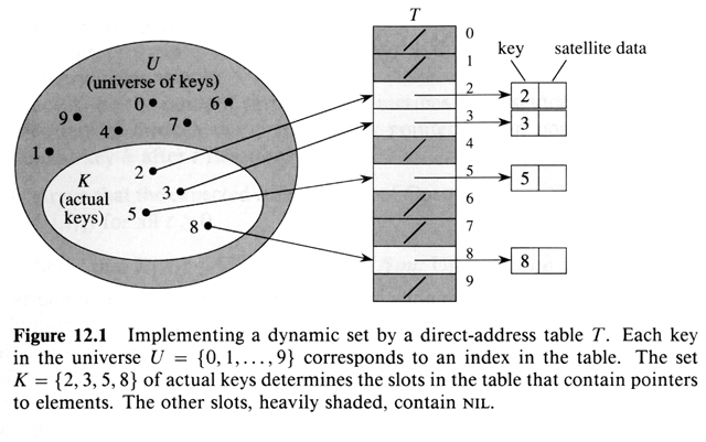
11.1 Direct-address Table(直接寻址表)

11.2 Hash Table

In direct-address Table, the element of key k is stored in slot k. In hash table, it is stored in slot h(k); h is hash function.

There is a problem in hash table: two keys may be mapped into a same slot. We call the situation collision. We have two ways to solve this. One is chaining(链接法), another is open addressing(开放寻址法).

Chaining

In chaining, the elements that hashed into same slot put in a linked list.

Load factor(装载因子) $\alpha$: giving a hash table that stored n elements, having m slots, $\alpha =n/m$. It means average stored elements’ number in a chain.

Simple uniform hashing(简单均匀散列): any given element have same possibility hashing to any one of m slots, regardless of where other elements are hashed.

11.3 Hash Function(散列函数)

Feature of good hash function: satisfy simple uniform hashing.

Tip: convert key to natural number

11.3.1 Division Method

Hash function: $h(k)=kmodm$
k is key, m is slots’ number. A prime that is not close to the power of 2, often a better choice for m.

11.3.2 Multiplication Method

The method has two steps. Step 1, key k multiplies constant A (0 < A < 1), extract fraction part of $kA$. Step 2, m multiplies Step 1 value, then round down.

Hash function is: $h(k)=\lfloor m(kAmod1)\rfloor$

$kAmod1$ gets fraction of $kA$, it mean $kA-\lfloor kA\rfloor$.

11.3.3 Universal Hashing(全域散列)

Universal hashing: randomly select a hash function from a group of hash functions. Strength: no matter select what keys as input, program can have a good average performance.

This is universal hashing function:
$h_{ab}(k)=((ak+b)\mathrm{m}\mathrm{o}\mathrm{d}p)\mathrm{m}\mathrm{o}\mathrm{d}m,a\in Z_p^{\ast },b\in Z_p$

All the function construct function family of universal hashing:
H p m = { h a b : a ∈ Z p ∗ ,   b ∈ Z p } \mathscr{H}_{pm}=\{h_{ab}:a \in Z_p^*, \space b \in Z_p\} Hpm​={hab​:a∈Zp∗​, b∈Zp​}

11.4 Open Addressing(开放寻址法)

For avoiding collision, open addressing need to probe(探查) hash table. Hash function of open addressing has second input parameter(probe number: start from 0), like this: $h(k,probeNumber)$.

For every key k, probe sequence(探查序列) $<h(k,0),h(k,1),\bullet \bullet \bullet ,h(k,m-1)>$ of open addressing is one arrangement of $<0,1,\bullet \bullet \bullet ,m-1>$

Below pseudo codes are hash insert and hash search by using open addressing.

HASH-INSERT(T, k)
1	i = 0
2	repeat
3		j = h(k, i)
4		if T[j] == NIL
5			T[j] = k
6			return j
7		else i = i + 1
8	until i == m
9	error "hash table overflow"

HASH-SEARCH(T, k)
1	i = 0
2	repeat
3		j = h(k, i)
4		if T[j] == k
5			return j
6		i = i + 1
7	until T[j] == NIL or i == m
8	return NIL

Deleting element in open addressing is more difficult. When we delete key from i slot, we can’t only put it NIL. Because if only do it, it will influence HASH-SEARCH. One way is: use a special value(like DELETED) to replace NIL. This only need to modify HASH-INSERT function a little. But if we use the special value DELETED, the search time will not only rely on load factor $\alpha$. So, if needing to delete key, common method is using chaining to solve collision.

There are 3 technologies to calculate probe sequence in open addressing: linear probing, quadratic probing, double hashing.

linear probing
given an ordinary hash function h ′ : U → { 0 , 1 , ⋅ ⋅ ⋅ , m − 1 } h': U\rightarrow\{0, 1, \cdot\cdot\cdot, m-1\} h′:U→{0,1,⋅⋅⋅,m−1}, call it auxiliary hash function(辅助散列函数), linear probing adopts followed hash function:
$h(k,i)=(h^{\prime }(k)+i)\mathrm{m}\mathrm{o}\mathrm{d}m,i=0,1,\cdot \cdot \cdot ,m-1$

Primary clustering(一次群集):

Quadratic probing
Quadratic probing adopts followed form hash function:
$h(k,i)=(h^{\prime }(k)+c_{1}i+c_2{i}^2)\mathrm{m}\mathrm{o}\mathrm{d}m$

$h^{\prime }(k)$ is auxiliary hash function, $c_{1}and{c}_2$ is positive auxiliary constant.

Secondary clustering(二次群集):

Double hashing
One of the best methods of open addressing. Double hashing adopts followed hash function:
$h(k,i)=(h_1(k)+i{h}_2(k))\mathrm{m}\mathrm{o}\mathrm{d}m,i=0,1,\cdot \cdot \cdot ,m-1$

$h_{1}and{h}_2$ are auxiliary hash function.

11.5 Perfect Hashing(完全散列)

static(静态): ones keys are stored in hash table, it don’t change.

Perfect hashing has some strengths:

1. Can find element in $\mathrm{O}(1)$ time complexity in worst case.
2. Expected space complexity: $\mathrm{O}(n)$

Perfect hashing can realize by using two-level hash. Every level use universal hashing(全域散列).

T is primary hash table, $S_j$ is secondary hash table(二次散列表). For assuring that secondary hash table doesn’t meet collision, the size $m_j$ of $S_j$ need to be square of the number $n_j$ of key hashed into slot j. ($m_j=n_j^2$)

Chapter 12: Binary Search Tree

12.1 What’s binary search tree

The key in binary search tree always satisfy followed property:
Assume $x$ is a node of binary search tree. if $y$ is a node of $x$'s left tree, then $y.key\le x.key$. if $y$ is a node of $x$'s right tree, then $y.key\ge x.key$

Inorder tree walk(中序遍历): print key value of subtree root between its left subtree value and its right subtree value.
Preorder tree walk(前序遍历): print key value of subtree root before its left subtree value and its right subtree value.
postorder tree walk(后序遍历): print key value of subtree root after its left subtree value and its right subtree value.

INORDER-TREE-WALK(x)	// complexity: Theta(n)
1	if x != NIL
2		INORDER-TREE-WALK(x.left)
3		print x.key
4		INORDER-TREE-WALK(x.right)

12.2 Query Binary Search Tree

Theorem 12.2: On a height $h$ binary search tree, operation SEARCH / MINIMUM / MAXIMUM / SUCCESSOR / PREDECESSOR on dynamic sets can complete in $\mathrm{O}(h)$.

SEARCH

TREE-SEARCH(x, k)	// recursive version
// x is tree root pointer
1	if x == NIL or k == x.key
2		return x
3	if k < x.key
4		return TREE-SEARCH(x.left, k)
5	else return TREE-SEARCH(x.right, k)

ITERATIVE-TREE-SEARCH(x, k)	// iterative version
1	while x != NIL and k != x.key
2		if k < x.key
3			x = x.left
4		else x = x.right
5	return x

MINIMUM and MAXIMUM

TREE-MINIMUM(x)
// x is subtree root pointer
1	while x.left != NIL
2		x = x.left
3	return x

TREE-MAXIMUM(x)
1	while x.right != NIL
2		x = x.right
3	return x

SUCCESSOR and PREDECESSOR

TREE-SUCCESSOR(x)
// x is a tree node
1	if x.right != NIL
2		return TREE-MINIMUM(x.right)
3	y = x.p
4	while y != NIL and x == y.right
5		x = y
6 		y = y.p
7	return y

TREE-PREDECESSOR(x)
1	if x.left != NIL
2		return TREE-MAXIMUM(x.left)
3	y = x.p
4	while y != NIL and x == y.left
5		x = y
6		y = y.p
7	return y

12.3 Insert and Delete

Theorem 12.3: On a height $h$ binary search tree, operation INSERT / DELETE on dynamic sets can complete in $\mathrm{O}(h)$.

INSERT

TREE-INSERT(T, z)
1	y = NIL
2	x = T.root
3	while x != NIL
4		y = x
5		if z.key < x.key
6			x = x.left
7		else x = x.right
8	z.p = y
9	if y == NIL
10		T.root = z	// tree T was empty
11	elseif z.key < y.key
12		y.left = z
13	else y.right = z

DELETE

TRANSPLANT(T, u, v)
1	if u.p == NIL
2		T.root = v
3	elseif u == u.p.left
4		u.p.left = v
5	else u.p.right = v
6	if v != NIL
7		v.p = u.p

TREE-DELETE(T, z)
1	if z.left == NIL
2		TRANSPLANT(T, z, z.right)
3	elseif z.right == NIL
4		TRANSPLANT(T, z, z.left)
5	else y = TREE-MINIMUM(z.right)
6		if y.p != z
7			TRANSPLANT(T, y, y.right)
8			y.right = z.right
9			y.right.p = y
10		TRANSPLANT(T, z, y)
11		y.left = z.left
12		y.left.p = y

12.4 Randomly Built Binary Search Tree

Definition: according to random order, insert n key to a initial empty tree.

Theorem 12.4: expected height of randomly built binary search tree with n different keys is $\mathrm{O}(\lg n)$.

Chapter 13: Red-Black Tree

Red-black tree is one of balanced binary search tree, it can guarantee that the time complexity of basic dynamic set operation is $\mathrm{O}(\lg n)$ in worst case.

13.1 Property of Red-Black Tree

It guarantees no one path is twice as long as other paths, so it’s approximate balanced.
Black-Height(黑高): $bh(x)$

Lemma 13.1: The height of a n internal nodes red-black tree is $2\lg (n+1)$ at most.

13.2 Rotation

The operation can keep property of binary search tree. Time complexity is $\mathrm{O}(1)$.

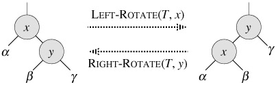
LEFT-ROTATE(T, x)
1	y = x.right	// set y
2	x.right = y.left	// turn y's left subtree into x's right subtree
3	if y.left != T.nil
4		y.left.p = x
5	y.p = x.p
6	if x.p == T.nil
7		T.root = y
8	elseif x == x.p.left
9		x.p.left = y
10	else x.p.right = y
11	y.left = x	// put x on y's left
12	x.p = y

13.3 INSERT

RB-INSERT(T, z)
1	y = T.nil
2	x = T.root
3	while x != T.nil
4		y = x
5		if z.key < x.key
6			x = x.left
7		else x = x.right
8	z.p = y
9	if y == T.nil
10		T.root = z	// tree T was empty
11	else if z.key < y.key
12		y.left = z
13	else y.right = z
14 	z.left = T.nil
15	z.right = T.nil
16	z.color = RED
17	RB-INSERT-FIXUP(T, z)

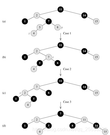
RB-INSERT-FIXUP(T, z)
1	while z.p.color == RED
2		if z.p == z.p.p.left
3			y = z.p.p.right
4			if y.color == RED
5				z.p.color = BLACK	// case 1
6				y.color = BLACK		// case 1
7				z.p.p.color = RED	// case 1
8				z = z.p.p			// case 1
9				continue
10			else if z == z.p.right
11				z = z.p				// case 2
12				LEFT-ROTATE(T, z)	// case 2
13			z.p.color = BLACK		// case 3
14			z.p.p.color = RED		// case 3
15			RIGHT-ROTATE(T, z.p.p)	// case 3
16		else(same as then clause with "right" and "left" exchanged)
17	T.root.color = BLACK

13.4 DELETE

RB-TRANSPLANT(T, u, v)
1	if u.p == T.nil
2		T.root = v
3	else if u == u.p.left
4		u.p.left = v
5	else u.p.right = v
6	v.p = u.p

RB-DELETE(T, z)
1	y = z
2	y-original-color = y.color
3	if z.left == T.nil
4		x = z.right
5		RB-TRANSPLANT(T, z, z.right)
6	else if z.right == T.nil
7		x = z.left
8		RB-TRANSPLANT(T, z, z.left)
9	else y = TREE-MINIMUM(z.right)
10		y-original-color = y.color
11		x = y.right
12		if y.p == z
13			x.p = y
14		else RB-TRANSPLANT(T, y, y.right)
15			y.right = z.right
16			y.right.p = y
17		RB-TRANSPLANT(T, z, y)
18		y.left = z.left
19		y.left.p = y
20		y.color = z.color
21	if y-original-color == BLACK
22		RB-DELETE-FIXUP(T, x)

RB-DELETE-FIXUP(T, x)
1	while x != T.root and x.color == BLACK
2		if x == x.p.left
3			w = x.p.right
4			if w.color == RED
5				w.color = BLACK			// case 1
6				x.p.color = RED			// case 1
7				LEFT-ROTATE(T, x.p)		// case 1
8				w = x.p.right			// case 1
9			if w.left.color == BLACK and w.right.color == BLACK
10				w.color = RED			// case 2
11				x = x.p					// case 2
				continue
12			else if w.right.color == BLACK
13				w.left.color = BLACK	// case 3
14				w.color = RED			// case 3
15				RIGHT-ROTATE(T, w)		// case 3
16				w = x.p.right			// case 3
17			w.color = x.p.color			// case 4
18			x.p.color = BLACK			// case 4
19			w.right.color = BLACK		// case 4
20			LEFT-ROTATE(T, x.p)			// case 4
21			x = T.root					// case 4
22		else (same as then clause with "right" and "left" exchanged)
23	x.color = BLACK

Concept
Persistent dynamic set(持久动态集合): when we update dynamic set, need to maintain past version.
AVL tree(AVL树): is a height balanced(高度平衡的) binary search tree. For every node $x$, the height difference of $x^{\prime }s$ left tree and $x^{\prime }s$ right tree is at most 1.
Treap tree(Treap树)：
B tree:

Chapter 14: Augmenting Data Structures(数据结构的扩张)

14.1 Dynamic Order Statistic

In chapter 9, we know that we can determine any order statistic in $\mathrm{O}(n)$ time for an unordered set. This section will introduce how to modify red-black tree to determine any order statistic in $\mathrm{O}(\lg n)$ time.

Order-statistic tree(顺序统计树): is simply a red-black tree with additional information stored in each node. Besides the usual red-black tree fields $x.key$, $x.color$, $x.p$, $x.left$, and $x.right$ in a node $x$, we have another field $x.size$. This field contains the number of (internal) nodes in the subtree rooted at x (including x itself), that is, the size of the subtree. If defined sentinel’s size is 0, that is, $T.nil.size=0$, then have equation:
$x.size=x.left.size+x.right.size+1$

Retrieving an element with a given rank

OS-SELECT(x, i)
1	r = x.left.size + 1
2	if i == r
3		return x
4	else if i < r
5		return OS-SELECT(x.left, i)
6	else return OS-SELECT(x.right, i - r)

Determining the rank of an element

OS-RANK(T, x)
1	r = x.left.size + 1
2	y = x
3	while y != T.root
4		if y == y.p.right
5			r = r + y.p.left.size + 1
6		y = y.p
7	return r

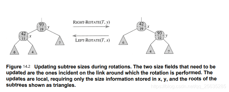
Maintaining subtree sizes

Insert operation:

We noted in section 13.3 that insertion into red-black tree consists of 2 phases. The first phase goes down the tree from the root, inserting the new node as a child of an existing node. The second phase goes up the tree, changing colors and ultimately performing rotations to maintain the red-black properties.

To maintain the subtree sizes in the first phase, we simply increment $x.size$ for each node $x$ on the path traversed from the root down toward the leaves. Since there are $\mathrm{O}(\lg n)$ nodes on the traversed path, the additional cost of maintaining the $size$ fields is $\mathrm{O}(\lg n)$.

In the second phase, the only structure changes to the underlying red-black tree are caused by rotations, of which there are at most 2. Moreover, a rotation is a local operation: it invalidates only the two size fields in the nodes incident on the link around which the rotation is performed. Referring to the code for LEFT-ROTATE(T,x) in Section 13.2, we add the following lines:

13	y.size = x.size
14	x.size = x.left.size + x.right.size + 1

Delete operation:

14.2 How to augment a data structure

Augmenting red-black tree

Theorem 14.1: let $f$ is a field that augmented a red-black tree T of n nodes, and suppose that the contents of $f$ for a node $x$ can be computed using only the information in nodes $x$, $x.left$ and $x.right$, including $x.left.f$ and $x.right.f$. Then, we can maintain the values of $f$ in all nodes of T during insertion and deletion without asymptotically affecting the $\mathrm{O}(\lg n)$ performance of these operations.

14.3 Interval trees

Intervals are convenient for representing events that each occupy a continuous period of time. We might, for example, wish to query a database of time intervals to find out what events occurred during a given interval. The data structure in this section provides an efficient means for maintaining such an interval database.

An interval tree is a red-black tree that maintains a dynamic set of elements, with each element x containing an interval $x.int$. Interval trees support the following operations:

INTERVAL-INSERT(T,x) adds the element x, whose int field is assumed to contain an interval, to the interval tree T.
INTERVAL-DELETE(T,x) removes the element x from the interval tree T.
INTERVAL-SEARCH(T,i) returns a pointer to an element x in the interval tree T such that $x.int$ overlaps interval i, or T.nil if no such element is in the set.

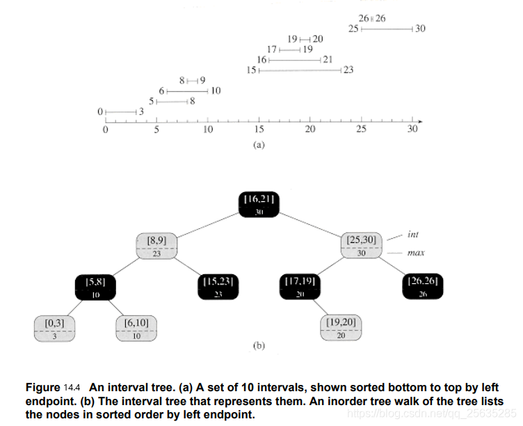
Interval tree is sorted by left endpoint.

Interval tree have some special fields with each node x:

• $x.int$ stores interval value. $x.int.low$ is low endpoint(低端点), $x.int.high$ is high endpoint(高端点).
• $x.max$ is the maximum of any interval endpoint stored in the subtree rooted at x.

INTERVAL-SEARCH(T, i)
1	x = T.root
2	while x != T.nil and i does not overlap x.int
3		if x.left != T.nil and x.left.max >= i.low
4			x = x.left
5		else x = x.right
6	return x