Machine Learning（7）Neural network —— Perceptrons

Machine Learning（7）Neural network —— Perceptrons

Chenjing Ding
2018/02/21

---

notation	meaning
g(x)	activate function
$x_n$	the n-th input vector (simplified as $x_i$ when n is not specified)
$x_{n_i}$	the i-th entry of $x_n$ (simplified as $x_i$ when n is not specified)
N	the number of input vectors
K	the number of classes
$t_n$	a vector with K dimensional with k-th entry 1 only when the n-th input vector belongs to k-th class, tn = (0,0,…1…0)
$y_j(x)$	the output of j-th output neural
$y(x)$	a output vector of input vector x; $y(x) = (y_1(x)...y_K(x))$
$W_{ji}^{\tau+1}$	the ($\tau+1$)-th update of weight $W_{ji}$
$W_{ji}^{\tau}$	the $\tau$-th update of weight $W_{ji}$
$\frac{\partial E(W)}{\partial W_{ij}^{(m)}}$	the gradient of m-th layer weight
$l_i$	the number of neural in i-th layer
$W_{ji}^{(mn)}$	the weight between layer m and n

---

1. two layers perceptron

1.1 construction

2 layers refers to output layer and input layer; the basic construction of 2 layers perceptron is as followed:

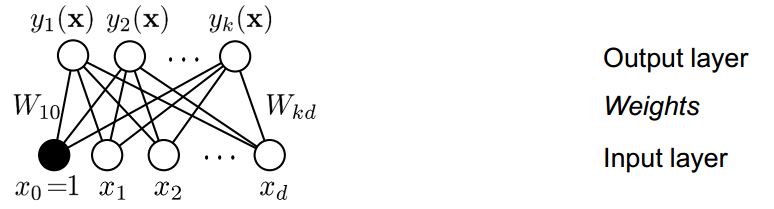
figure1 the construction of 2 layers perceptron

input layer:
d neural, d is the dimensional of an input vector x; The input layer can applied with non-linear basic functions $\phi(x)$.

Weights:
$W_{ji}$, j is the index of neural in output layer;i is the index of neural in input layer;

Output layer:
There are k classes, so there are k output functions. The output layer can applied with activate function g(x).

$$\exists y_i(x) > y_j(x), \forall j \neq i \Rightarrow input\ data\ x \in C_i \\ linear\ output:y_j(x) = \sum_{i=0}^d W_{ji}*x_i \ \ or\ \sum_{i=0}^d W_{ji}*\phi(x_i) \\ nonlinear\ output:y_j(x) =g( \sum_{i=0}^d W_{ji}*x_i) \ \ or \ \ g( \sum_{i=0}^d W_{ji}*\phi(x_i))$$

1.2 Learning: How to get $W_{ji}$

Gradient descent with sequential updating can be used to minimize the error function E(W) to adjust weights.

step1: set up an error function E(W);
if we use L2 loss,

$$E_n(W) = \frac{1}{2}(\ y(x_n) - t_n)^2 = \frac{1}{2} \sum_{ l=1}^K (y_l(x_n) - {t_n}_l)^2\\ = \frac{1}{2} \sum_{ l=1}^K (\sum_{m=0}^d Wlm*\phi(x_m) - {t_n}_l)^2$$
step2: calculate $\frac{\partial E_n(W)}{ \partial W_{ji}}$;
$$\frac{\partial E_n(W)}{ \partial W_{ji}} = \sum_{ l=1}^K [(y_l(x_n) - {t_n}_l) *\frac{\partial y_l(x_n)}{ \partial W_{ji}}] = (\ y_j(x_n) - {t_n}_j) *\phi(x_i)$$
step3: sequential updating, $\eta$ is the learning rate;
$$W_{ji}^{\tau + 1} = W_{ji}^\tau - \eta \frac{\partial E_n(W)}{ \partial W_{ji}} \\ = W_{ji}^\tau - \eta [ (\ y_j(x_n) - {t_n}_j) *\phi(x_i)] \ \ (Delta\ rule / LMS\ rule)$$
Thus, perceptron learning corresponds to Gradient Descent of a quadratic error function.

1. effor function more details:
2. sequential updating and delta rule:
3. Gradient descent

1.3 properties of 2 layers perceptron

1. it can only represent the linear function since

   $$y_j(x) = \sum_{i=0}^d W_{ji}*x_i \ \ or\ \sum_{i=0}^d W_{ji}*\phi(x_i)$$ the discriminant boundary is always linear in input space x or input space $\phi(x)$ when input layer applied with $\phi(x)$, to be specific, the boundary can be a line, a plane and can not be a curve and so on. However, multi layers perceptron with hidden units can represent any continuous functions.$\Rightarrow$ 2. multi layers perceptron

2. $\phi(x)$ and $g(x)$ are given before; They are fixed functions.

3. There is always bias item in the linear discriminant function; (y = ax+b，b is the bias item and it has nothing to do with input x), thus the input layer always have d+1 input neural and the $x_0$ is always 1, in a result $y = ax_1 + bx_0 ,x_1 = x,d = 1$;

2 multi layers perceptron

There are some hidden layers between input layer and output layer.
For example, perceptron with one hidden layer as followed,

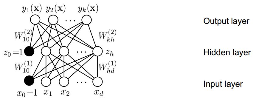
figure2 the construction of multi layers perceptron

output:

$$y_k(x) = g^{(2)}[\sum_{i=0}^h W_{ki}^{(2)}g^{(1)}[\sum_{j=0}^d W_{ij}^{(1)}x_j]]$$
In 1.2 we know how to learn the weight of 2 layers perceptron. As the same way, for multi layers, we also need to find the error function and using Gradient Decent to update all weights, but computing the gradient is more complex. So here are 2 main steps:

step1: computing the gradient $\Rightarrow$ 2.1Backpropogation
step2: adjusting the weight in the direction of gradient, same as 1.2 step3, we well later focus on some optimization techniques to improve the performance $\Rightarrow$ Machine Learning（7）Neural network–optimization techniques

2.1 Backpropagation

2.1.1 How to use backpropagation

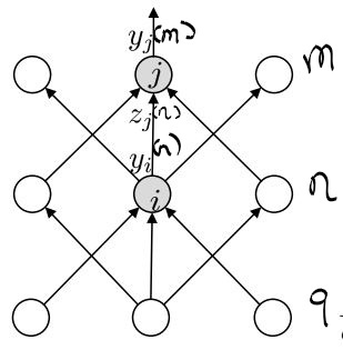
figure3 the construction of multi layers perceptron

if the id of layer is m, n and q form top to bottom, the number of neural in each layer is $l_m,l_n$and $l_q$; between 2 layers, the above layer is always the output layer with index of neural j and similarly, the bottom layer is always the input layer with i;

Our goal is to obtain the gradient of $\frac{\partial E(W)}{\partial Wji^{(mn)}}$:

$$y_j^{m} = g(z_{j}^{(n)})\\z_{j} ^{(n)}=\sum_{i =1 }^{l_n} W_{ji}^{(mn)}*y_i^{(n)} \\ \frac{\partial E(W)}{\partial Wji^{(mn)}} = \frac{\partial E(W)}{\partial y_j^{(m)} } \frac{ \partial y_j^{(m)} }{\partial Wji^{(mn)}} = \frac{\partial E(W)}{\partial y_j^{(m)} } \frac{\partial y_j^{(m)}}{\partial z_j^{(n)}} \frac{\partial z_j^{(n)}} {\partial Wji^{(mn)}}$$ thus here are 3 gradients need to be computed to get the result.
$$\frac{\partial E(W)}{\partial z_j^{(n)} }= \frac{\partial E(W)}{\partial y_j^{(m)} } \frac{\partial y_j^{(m)}}{\partial z_j^{(n)}} = \frac{\partial E(W)}{\partial y_j^{(m)} } g' \\\frac{\partial z_j^{(n)}} {\partial Wji^{(mn)}} = y_i^{(n)} \Rightarrow \frac{\partial E(W)}{\partial Wji^{(mn)}} = \frac{\partial E(W)}{\partial y_j^{(m)} } g' *y_i^{(n)} \\ \frac{\partial E(W)}{\partial y_i^{(n)} } = \sum_{j=1}^{l_m} \frac{\partial E(W)}{\partial z_j^{(n)} }\frac{ \partial z_j^{(n)}}{\partial y_i^{(n)} } = \sum_{j=1}^{l_m} W_{ji}^{(mn)} \frac{\partial E(W)}{\partial z_j^{(n)} }$$ Thus, 3 gradients above needs to be calculated between every 2 adjacent layers. Once we got the $\frac{\partial E(W)}{\partial y_j^{(m)} }$ from the above m+1 layer then we can obtain $\frac{\partial E(W)}{\partial Wji^{(mn)}}$ and calculate the $\frac{\partial E(W)}{\partial y_i^{(n)} }$ to prepare the next layer down calculation for $\frac{\partial E(W)}{\partial z_j^{(q)} }$ ; It is called reverse-mode differentiation.

2.1.2 Why use backpropagation with reverse-mode differentiation

For all adjacent layers m and n, There are 2 ways to calculate $\frac{\partial E(W)}{\partial W_{ij}^{(mn)}}$. To simplify, suppose we want to calculate $\frac{\partial Z }{\partial X}$, one way is to apply operator$\frac{\partial }{\partial X}$ to every node, which is called Forward-Mode Differentiation. The other way is to apply operator$\frac{\partial Z }{\partial }$ called reverse-mode differentiation;

*figure4 computation graph* *1: Forward - Mode - Differentiate*

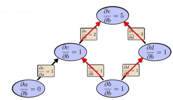*figure5 Forward - Mode - Differentiate computation graph*

$$\frac{\partial e }{\partial b} = \frac{\partial e }{\partial c} \frac{\partial c}{\partial b} + \frac{\partial e }{\partial d} \frac{\partial d}{\partial b} = 5$$ Visiting all red lines only get one gradient which is not efficient.

Forward-mode-differentiate apply operator$\frac{\partial }{\partial b}$ to every node, in our cases, the operator is $\frac{\partial }{\partial y_j^{(m)}}$ if the goal is to obtain $\frac{\partial E(W)}{\partial W_{{j_m}i}^{(m \ m-1)}}$;the id of first layer down is 0;

$$\frac{\partial E(W)}{\partial W_{{j_1}i}^{(10)}} = \frac{\partial E(W)}{\partial y_{j_1}^{(1)}}\frac{\partial y_{j_1}^{(1)}} {\partial W_{i{j_1}}^{(10)}} =\frac{\partial E(W)}{\partial y_{j_1}^{(1)}}\frac{\partial y_{j_1}^{(1)}} {\partial W_{{j_1}i}^{(10)}}\\= [\sum_{j_2} \frac{\partial E(W)}{\partial y_{j_2}^{(2)}} \frac{\partial y_{j_2}^{(2)}} {\partial y_{j_1}^{(1)}} ]\frac{\partial y_{j_1}^{(1)}} {\partial W_{{j_1}i}^{(10)}} \\= [\sum_{j_3}\sum_{j_2} \frac{\partial E(W)}{\partial y_{j_3}^{(3)}} \frac{\partial y_{j_3}^{(3)}} {\partial y_{j_2}^{(2)}}\frac{\partial y_{j_2}^{(2)}} {\partial y_{j_1}^{(1)}} ]\frac{\partial y_{j_1}^{(1)}} {\partial W_{{j_1}i}^{(10)}}\\ = [\sum_{j_{q-1}}...\sum_{j_3}\sum_{j_2} \frac{\partial E(W)}{\partial y_{j_{q-1}}^{(q-1)}} \frac{\partial y_{j_{q-1}}^{(q-1)}} {\partial y_{j_{q-2}}^{(q-2)}}...\frac{\partial y_{j_2}^{(2)}} {\partial y_{j_1}^{(1)}} ]\frac{\partial y_{j_1}^{(1)}} {\partial W_{{j_1}i}^{(10)}}$$
thus we need to visit every layer only to get $\frac{\partial E(W)}{\partial W_{{j_1}i}^{(10)}}$, when it comes to $\frac{\partial E(W)}{\partial W_{{j_1 }i +1}^{(10)}}$,we need to visit every layer again!

2: reverse-mode differentiation

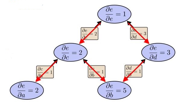
figure6 Reverse-mode differentiation computation graph

From the graph above, only one pass we know $\frac{\partial e }{\partial }$ to all nodes. It is more efficient than Forward-mode-differentiate.
Reverse-mode differentiation apply $\frac{\partial e }{\partial }$ to every node, in our case, it is $\frac{\partial E(W) }{\partial }$ ;That is to say, $\frac{\partial E(W)}{\partial y_{j_{q-1}}^{(q-1)}},\frac{\partial E(W)}{\partial y_{j_{q-2}}^{(q-2)}}...\frac{\partial E(W)}{\partial y_{j_{1}}^{(1)}}$ are calculated in order.
Then $\frac{\partial E(W)}{\partial W_{j_{q-1} i_{q-1}}^{(q-1,q-2)}},\frac{\partial E(W)}{\partial W_{j_{q-2},i_{q-2}}^{(q-2,q-3)}}...\frac{\partial E(W)}{\partial W_{j_1 i_1}^{(1,0)}}$are also obtained ; As mentioned above, $i_m$ is the id of neural in m-th layer when this layer is input layer, $i_m$can be 0 to $l_m$; $j_m$ is in similar way.

From all above, Reverse-mode differentiation can compute all derivatives in one single pass, that is why we use Back-propagation with reverse-mode differentiation;

Next topic will introduce some optimization techniques and how to implement these ideas with python.