Neural Networks and Deep Learning 【编程笔记】

class 2 : Logistic Regression with a Neural Network mindset

1. 提取数据（图片）维度

m_train = train_set_x_orig. shape[0]

num_px = train_set_x_orig .shape[1]

print ("train_set_x shape: " + str(train_set_x_orig.shape))

Each image is of size: (64, 64, 3)train_set_x shape: (209, 64, 64, 3)

2. 将矩阵转为列向量堆叠

train_set_x_flatten = train_set_x_orig. reshape(train_set_x_orig.shape[0], -1 ).T

train_set_x = train_set_x_flatten/255 数据标准化

3. 初始化W，b

initialize_with_zeros(dim)

w = np.zeros((dim,1))

b = 0

注意用assert检查数据类型和矩阵维度

assert(w.shape == (dim, 1))

assert(isinstance(b, float) or isinstance(b, int))

4. 前向传播

def propagate(w, b, X, Y)：

m = X.shape[1] #注意样本数目所在维度！！

A = sigmoid(np.dot(w.T,X)+b) # X保持维度不变！

cost = -np.sum(Y*np.log(A)+(1-Y)*np.log(1-A))/m # 注意sum用法，最后除以样本总量！

dw = np.dot(X,(A-Y).T)/m

db = np.sum(A-Y)/m

5. 多次迭代

for i in range(num_iterations):

grads, cost = propagate(w, b, X, Y)

w = w-dw*learning_rate

b = b-db*learning_rate

------------------------------------------------------------------------------------------

class 3 : Planar data classification with one hidden layer v5

1. 作图&检查矩阵维度

plt.scatter(X[0, :], X[1, :], c=Y, s=40, cmap=plt.cm.Spectral)

2. 各层维度定义

def layer_sizes(X, Y)：

n_x = X.shape[0] # size of input layer

n_h = 4

n_y = Y.shape[0]

3. 参数初始化

def initialize_parameters(n_x, n_h, n_y):

W1 = np.random.randn( n_h,n_x)* 0.01

b1 = np.zeros((n_h,1))

W2 = np.random.randn( n_y,n_h)* 0.01

b2 = np.zeros((n_y,1))

4. 前向传播

def forward_propagation(X, parameters):

Z1 = np.dot(W1,X)+b1

A1 = np. tanh(Z1)

Z2 = np.dot(W2, A1)+b2 # 这里注意不要写成X!!

A2 = sigmoid(Z2)

5. 损失计算

def compute_cost(A2, Y, parameters):

logprobs = np.multiply(np.log(A2),Y)+np.multiply(np.log(1-A2),(1-Y))

cost = - 1/m*np.sum(logprobs)

cost = np.squeeze(cost)

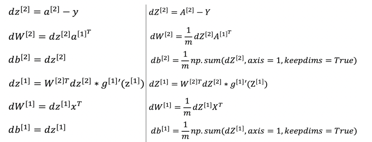
6.反向传播

dZ2 = A2-Y

dW2 = 1/m*np.dot(dZ2,A1.T)

db2 = 1/m*np.sum(dZ2,axis=1,keepdims=True)

dZ1 = np.dot(W2.T,dZ2)* (1 - np.power(A1, 2))

dW1 = 1/m*np.dot(dZ1,X.T)

db1 = 1/m*np.sum(dZ1,axis=1,keepdims=True)

7. 参数更新

------------------------------------------------------------------------------------------

class 4 : Building your Deep Neural Network - Step by Step

1. 参数初始化

initialize_parameters(n_x, n_h, n_y) 返回parameters，存入各层的W,b

initialize_parameters_deep(layer_dims)

L = len(layer_dims)

for l in range(1, L):

parameters['W' + str(l)] = np.random.randn(layer_dims[l], layer_dims[l-1]) * 0.01 【注意层数和各层元素初始化之间的关系】

parameters['b' + str(l)] = np.zeros((layer_dims[l], 1))

2. 前向传播

def linear_forward(A, W, b)：

Z = np.dot(W,A)+b

cache = (A, W, b) 将该层的输入与参数保存下来

return Z, cache

def linear_activation_forward(A_prev, W, b, activation):

Z, linear_cache = linear_forward(A_prev,W,b)

A, activation_cache = sigmoid(Z) activation_cache里存的就是Z

cache = (linear_cache, activation_cache) 注意这时候cache存的是两个部分

return A, cache

def L_model_forward(X, parameters):

A = X

L = len(parameters) // 2 # number of layers in the neural network

for l in range(1, L):

A_prev = A

A, cache = linear_activation_forward(A_prev, parameters["W"+str(l)], parameters["b"+str(l)], 'relu')

caches.append(cache)

AL, cache = linear_activation_forward(A,parameters["W"+str(L)], parameters["b"+str(L)], 'sigmoid')

caches.append(cache)

return AL, caches

3. 损失计算

def compute_cost(AL, Y):

m = Y.shape[1]

cost = -1/m*np.sum(np.multiply(Y,np.log(AL))+np.multiply(1-Y,np.log(1-AL)))

cost = np.squeeze(cost)

return cost

4. 反向传播 【难点！重点！】

def linear_backward(dZ, cache):

A_prev, W, b = cache

m = A_prev.shape[1]

dW = 1/m*np.dot(dZ,A_prev.T)

db = 1/m*np.sum(dZ,axis=1,keepdims=True)

dA_prev = np.dot(W.T,dZ)

return dA_prev, dW, db

def linear_activation_backward(dA, cache, activation):

linear_cache, activation_cache = cache

if activation == "relu":

dZ = relu_backward(dA, activation_cache)

dA_prev, dW, db = linear_backward(dZ, linear_cache)

elif activation == "sigmoid":

dZ = sigmoid_backward(dA, activation_cache)

dA_prev, dW, db = linear_backward(dZ, linear_cache)

return dA_prev, dW, db

def L_model_backward(AL, Y, caches):

dAL = - (np.divide(Y, AL) - np.divide(1 - Y, 1 - AL))

current_cache = caches[L-1]

grads["dA" + str(L)], grads["dW" + str(L)], grads["db" + str(L)] = linear_activation_backward(dAL, current_cache, 'sigmoid')

for l in reversed(range(L-1)):

current_cache = caches[l]

dA_prev_temp, dW_temp, db_temp = linear_activation_backward(grads["dA" + str(l+2)], current_cache, 'relu')

grads["dA" + str(l + 1)] = dA_prev_temp

grads["dW" + str(l + 1)] = dW_temp

grads["db" + str(l + 1)] = db_temp

return grads

这个函数应该是有错误在的，最后这一部分没有得分，推导了一下反向求导的逻辑，大致有了了解。

目前比较困惑cache里每一层的数据所存的下标到底是什么，感觉这里有些混乱，应该是导致出错的原因；另外就是对于整个求导的逻辑确实需要再熟悉、明确一下。

5. 参数更新

def update_parameters(parameters, grads, learning_rate):

L = len(parameters) // 2 # number of layers in the neural network

for l in range(L):

parameters["W" + str(l+1)] = parameters["W" + str(l+1)]- learning_rate*grads["dW"+str(l+1)]

parameters["b" + str(l+1)] = parameters["b" + str(l+1)]- learning_rate*grads["db"+str(l+1)]

return parameters

------------------------------------------------------------------------------------------

Deep Neural Network for Image Classification: Application

这一部分基本就是把前面写过的各种函数整体梳理应用一下，贴对函数名字，放对参数就可以，不再赘述。