感知机算法原理与多种python实现方式结果可视化

最新推荐文章于 2023-11-28 23:33:09 发布

桉夏与猫

最新推荐文章于 2023-11-28 23:33:09 发布

阅读量2.4k

点赞数 3

分类专栏：深度学习 python 文章标签：算法 python 机器学习深度学习人工智能

本文链接：https://blog.csdn.net/qq_28790663/article/details/115528845

版权

python 同时被 2 个专栏收录

25 篇文章 2 订阅

订阅专栏

深度学习

12 篇文章 5 订阅

订阅专栏

感知机(perceptron)算法

二分类模型、线性分类模型、判别模型

感知机(perceptron)是根据输入数据的特征向量x，对其进行二分类的一种线性分类模型。

感知机的输出与输出：

输入（input）	输出（output）
实例的特征向量	实例的类别（取值为+1或-1）

感知机是一个分类器，对于输入空间内的实例划分为正负两类超平面，属于判别模型！（比如：有两组数据作为训练集，其中的类别是A和B，在训练完成后，通过给定一个测试数据，感知器能够将其分成A或者B）

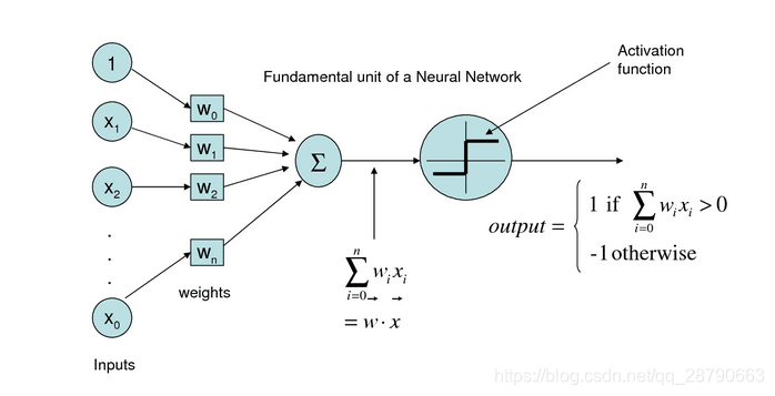
感知机模型

感知机模型实际上是一个超平面：

$f(x) = sign(wx+b)$

其中 $x\in R^{n}$ , $w\in R^{n}$ , $b\in R$

当 $wx+b>0$ 时，模型将该样本分为正类

当 $wx+b>0$ 时，模型将该样本分为负类

(图中有错误，最下面的 $x_{0}$ 应该是 $x_{n}$ )

感知器包括多个输入节点，从 $x_{1}$ 到 $x_{n}$ ，有多个权重矩阵 $w_{0}$ 到 $w_{n}$ 。一个输出节点O，激活函数使用sigh函数，最后输出的值为1或者-1

学习策略：

令 M 代表样本点被误分的集合。

所有的被误分类的点都满足： $yi(wi+b)<0$

损失函数为： $L(w,b) = \sum_{xi \in M}yi(w xi+b)$

优化目标是损失最小化，含义为：最小化误分类点到决策面的距离！

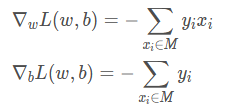
学习算法（优化算法）

随机梯度下降算法（stochastic gradient descent）——每次选取一个被误分类的点，计算损失函数并进行参数更新。

计算梯度：

参数更新：

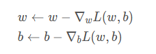
即：

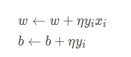
感知器学习规则

输入训练样本X和初始的权重矩阵W，将其进行向量的点乘，按后将求和的结果作用于激活函数sigh（），得到预测输出O，根据预测输出值和目标之间的差距error来调整权重向量W。如此反复，直到W调整到合适的结果。

使用python手动实现感知器模型：

数据集：sklearn中的鸢尾花（iris）数据集

相关任务：分类

实例的个数：150个

特征的个数：4个

有无缺失值：无

Abstract: Famous database; from Fisher, 1936

数据集介绍：iris数据集是由Fisher在1936年整理，包含四个特征：

Speal.Length(花萼长度)

Speal.Width（花萼宽度）

Petal.Length（花瓣长度）

Petal.Width（花瓣宽度）

四个特征的类型都为浮点型，单位是厘米。

类别共有三类：

Iris Setosa（山鸢尾）

Iris Versicolour（杂色鸢尾）

Iris Virginica(维吉尼亚鸢尾)

第一个实验Sklearn的Iris数据集拿出两个类别，并以[Speal.Length,Speal.Width]做为特征：

import numpy as np
import pandas as pd
import matplotlib.pyplot as plt
from sklearn.datasets import load_iris
def display(df,x_points,y_):
    fig = plt.figure()
    ax1= fig.add_subplot(1,2,1)
    ax2 = fig.add_subplot(1,2,2)
    fig.tight_layout()  # 设置默认的间距
    #选取1-50作为第一类，50-100作为第二类
    ax1.scatter(df[:50]['sepal length'],df[:50]['sepal width'],color='blue',label='0')
    ax1.scatter(df[50:100]['sepal length'],df[50:100]['sepal width'],color='orange',label='1')
    ax1.set_xlabel('sepal length')
    ax1.set_ylabel('sepal width')
    ax1.legend()
    #可视化展示
    ax2.plot(x_points, y_)
    ax2.scatter(df[:50]['sepal length'],df[:50]['sepal width'], color='blue', label='0')
    ax2.scatter(df[50:100]['sepal length'],df[50:100]['sepal width'] , color='orange', label='1')
    ax2.set_xlabel('sepal length')
    ax2.set_ylabel('sepal width')
    ax2.legend()
    fig.show()
def load_data():
    # 加载iris数据集
    iris = load_iris()
    # 转换成df格式，然后将列名设置为对应的标签名
    df = pd.DataFrame(iris.data, columns=iris.feature_names)
    df['label'] = iris.target
    df.columns = ['sepal length', 'sepal width', 'petal length', 'petal width', 'label']
    # 为了方便可视化，只使用sepal length 和 sepal width作为特征
    return df
class Perceptron():
    def __init__(self):
        self.w = np.ones(len(data[0])-1 , dtype=np.float32)
        self.b = 0
        self.l_rate = 0.1
        self.epoch = 1000
    #定义符号函数
    def sign(self,x,w,b):
        y = np.dot(x, w) + b
        return y
    def fit(self,x_train,y_train):
        error_count=0
        for _ in range(self.epoch):
            for i in range(len(x_train)):
                xi = x_train[i]
                yi = y_train[i]
                #如果当前节点分类错误
                if yi * self.sign(xi,self.w,self.b) <= 0:
                    self.w += self.l_rate * np.dot(xi,yi)
                    self.b += self.l_rate * yi
                    error_count += 1
            # print('w='+str(self.w)+',b='+str(self.b))
if __name__ == '__main__':
    df = load_data()
    #选取前100个数据，选择的列为第0列，第1列，最后一列（标签）
    data = np.array(df.iloc[:100,[0,1,-1]])
    X,y = data[:,:-1],data[:,-1]

    #对标签进行变换，由于感知机只能分类两类，输出值为1或-1，所以需要把0标签转换为-1
    y = np.array([1 if label==1 else -1 for label in y])
    perception =Perceptron()
    perception.fit(X,y)
    # 可视化超平面
    x_points = np.linspace(4, 7, 10)  # linspace返回固定间隔的数据
    # 误差分类点到超平面的距离
    y_ = -(perception.w[0] * x_points + perception.b) / perception.w[1]
    display(df,x_points,y_)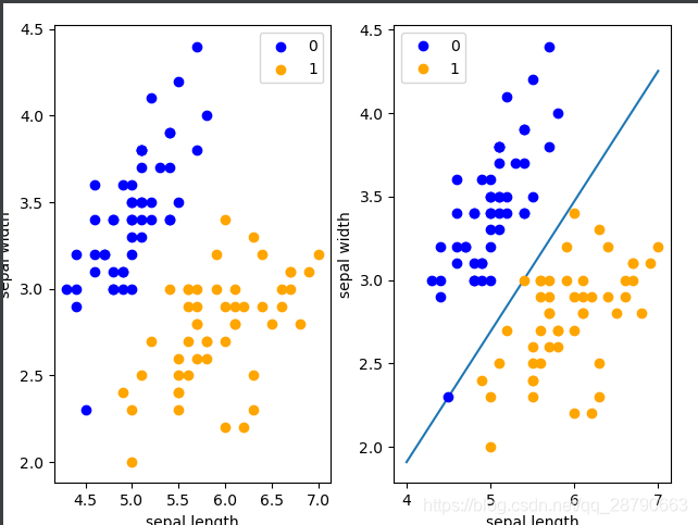

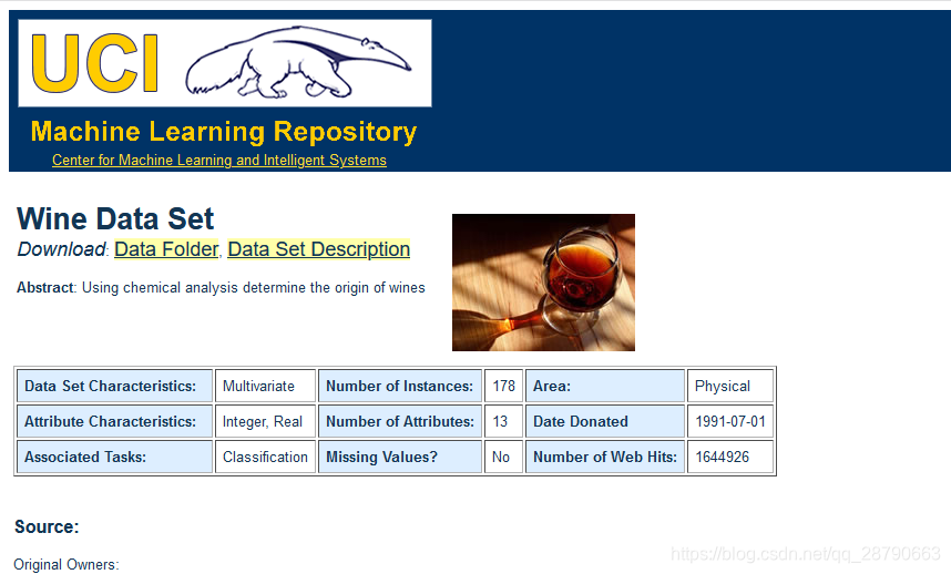
接下来在红酒数据集上进行试验，不再进行可视化，而是使用多个评价指标进行试验：

"""
__author__:shuangrui Guo
__description__:
"""
import numpy as np
import pandas as pd
import matplotlib.pyplot as plt
from sklearn.linear_model import Perceptron
from sklearn.metrics import accuracy_score
from sklearn.metrics import f1_score
from sklearn.metrics import precision_score
from sklearn.metrics import recall_score
from sklearn.metrics import roc_auc_score
#加载红酒数据集
def load_wine_data(file_path):
    labels = []
    features = []
    with open(file_path,'r',encoding='utf-8') as f:
        for line in f.readlines():
            content=line.strip().split(',')
            labels.append(content[0])
            features.append(list(map(float,content[1:])))
    df = pd.DataFrame(features)
    df.columns =['Alcohol','Malic acid','Ash','Alcalinity of ash','Magnesium','Total phenols','Flavanoids','Nonflavanoid phenols','Proanthocyanins','Color intensity','Hue','OD280/OD315 of diluted wines','Proline']
    labels = pd.DataFrame(labels,columns=['label'])
    data = pd.concat((df,labels),axis=1)
    return data



if __name__ == '__main__':
    wine_file_path = './wine.data'
    data = load_wine_data(wine_file_path)
    #取前130个数据（前130行数据包括两类）
    features = np.array(data.iloc[:130,:])
    X_train = np.concatenate([features[:49,:-1], features[60:120,:-1]], axis=0)
    y_train = np.concatenate([features[:49,-1],features[60:120,-1]],axis=0)
    y_train= np.array([1 if label =='1' else -1 for label in y_train])
    #X_train,y_train = features[:59,:-1]+features[:,:-1],features[:59,-1]+features[:,-1]
    X_test=np.concatenate([features[49:59,:-1], features[120:130,:-1]], axis=0)
    y_test = np.concatenate([features[49:59,-1],features[120:130,-1]], axis=0)
    y_test= np.array([1 if label =='1' else -1 for label in y_test])
    perceptron = Perceptron(fit_intercept=False,max_iter=1000,shuffle=True)
    perceptron.fit(X_train,y_train)
    y_pre = perceptron.predict(X_test)

    print('测试集准确率为:',accuracy_score(y_test,y_pre))
    print('测试集的F1值为:',f1_score(y_test,y_pre))
    print('测试集的precision_score为：',precision_score(y_test,y_pre))
    print('测试集的recall_score为：',recall_score(y_test,y_pre))
    print('测试集的roc_auc_score值为:', roc_auc_score(y_test, y_pre))

测试集准确率为: 0.95
测试集的F1值为: 0.9523809523809523
测试集的precision_score为： 0.9090909090909091
测试集的recall_score为： 1.0
测试集的roc_auc_score值为: 0.9500000000000001

桉夏与猫

关注

3
点赞
踩
25

收藏

觉得还不错? 一键收藏
1
评论
感知机算法原理与多种python实现方式结果可视化

感知器算法什么是感知器：感知器是根据输入数据的特征向量x，对其进行二分类的一种线性分类模型。f(x)=sign(w⋅x+b)感知器是一个分类器，对于输入空间内的实例划分为正负两类超平面，属于判别模型！比如：有两组数据作为训练集，其中的类别是A和B，在训练完成后，通过给定一个测试数据，感知器能够将其分成A或者B感知器模型：(图中有错误，最下面的x0应该是xn)感知器包括多个输入节点，从x1-xn，有多个权重矩阵W0-Wn。一个输出节点O，激活函数使用Sigh函数，最后输出的
复制链接

扫一扫