生成对抗网络介绍（附TensorFlow代码）

生成对抗网络介绍（附TensorFlow代码）

最近在生成模型方面研究非常热门（例如，参见OpenAI博客文章）。这些模型可以学习创建与我们提供的数据类似的数据。这个背后的直觉是，如果我们能够得到一个模型来写出高质量的新闻文章，那么一定也会从中学到很多关于新闻的文章。换句话说，这个模型也应该有一个很好的新闻报道的内部表现形式。然后我们可以用这个表示来帮助我们完成其他相关的任务，比如按主题对新闻文章进行分类。

实际上，培养模型来创建这样的数据并不容易，但近年来一些方法开始工作得很好。一种这样的有希望的方法是使用生成对抗网络（GAN）。 Facebook上最着名的深度学习研究员和AI研究主任Yann LeCun最近引用GANs作为深度学习最重要的新发展之一：

“There are many interesting recent development in deep learning…The most important one, in my opinion, is adversarial training (also called GAN for Generative Adversarial Networks). This, and the variations that are now being proposed is the most interesting idea in the last 10 years in ML, in my opinion.” – Yann LeCun

本文的其余部分将更详细地描述GAN公式，并提供一个使用GAN来解决问题的简单示例（带有TensorFlow中的代码）。

Discriminative vs. Generative models

在研究GAN之前，让我们简要回顾一下生成模型（generative model）和判别模型（discriminative model）的区别：

• 判别模型：学习将输入数据（x）映射到某个期望输出类别标签（y）的函数。用概率术语，他们直接学习条件分布P（y | x）。
• 生成模型：试图同时学习输入数据和标签的联合概率，即P（x，y）。这可以通过贝叶斯规则转换为P（y | x）进行分类，但是生成能力也可以用于其他方面，例如创建可能的新（x，y）样本。

两种类型的模型都是有用的，但是生成模型比歧视模型有一个有趣的优势 - 即使没有标签，他们也有可能理解和解释输入数据的基本结构。当处理现实世界中的数据建模问题时，这是非常可取的，因为未标记的数据当然是丰富的，但获得标记的数据往往是昂贵的。

Generative Adversarial Networks

GAN是一个有趣的想法，由Ian Goodfellow（现在在OpenAI）领导的蒙特利尔大学的一组研究人员于2014年首次提出。 GAN背后的主要思想是有两个竞争的神经网络模型。 一个将噪声作为输入并生成样本（所以称为生成器）。 另一个模型（称为鉴别器）从发生器和训练数据中接收样本，并且必须能够区分这两个源。 这两个网络连续游戏，发生器正在学习产生越来越多的现实样本，而鉴别器正在学习如何更好地区分生成的数据和真实的数据。 这两个网络是同时训练的，希望这个竞争将使生成的样本与真实的数据无法区分。

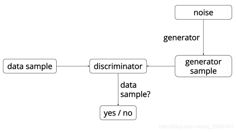
这里经常用到的比喻是，“生成器”就像一个试图制造伪造材料的伪造者，“鉴别器”就像是警方试图检测伪造的物品。这种说法也似乎有点让人想起强化学习，其中“生成器”接收来自“鉴别器”的奖励信号，从而知道所产生的数据是否准确。然而，与GAN的主要区别在于，我们可以将梯度信息从“鉴别器”反向传播回“生成器”网络，因此“生成器”知道如何调整其参数以产生可以欺骗“鉴别器”的输出数据。

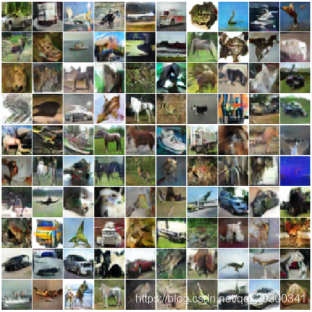
到目前为止，GAN主要应用于图像建模。他们现在在图像生成任务中产生了优异的结果，生成的图像比那些“基于最大似然训练目标方法训练”的图像要清楚得多。以下是由GAN生成的图像的一些示例：

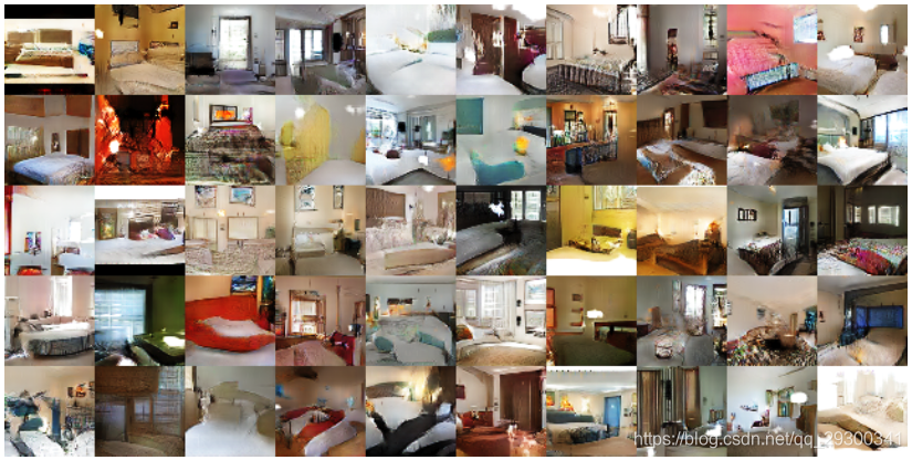
Generated bedrooms. Source: “Unsupervised Representation Learning with Deep Convolutional Generative Adversarial Networks” https://arxiv.org/abs/1511.06434v2

Approximating a 1D Gaussian distribution

为了更好地理解这一切是如何工作的，我们将使用GAN来解决TensorFlow中的玩具问题 - 学习逼近一维高斯分布。 这是基于Eric Jang的一个类似目标的博客文章。 我们演示的完整源代码可以在Github上找到（https://github.com/AYLIEN/gan-intro），在这里我们只关注代码中一些更有趣的部分。

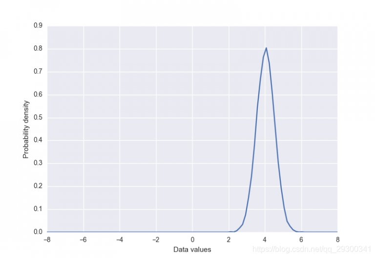
首先我们创建“真实”的数据分布，一个简单的高斯均值为4，标准差为0.5。 它有一个样本函数，用于从分布中返回给定数量的样本（按值排序）。

class DataDistribution(object):
    def __init__(self):
        self.mu = 4
        self.sigma = 0.5

    def sample(self, N):
        samples = np.random.normal(self.mu, self.sigma, N)
        samples.sort()
        return samples

我们将尝试学习的数据分布如下所示：

我们还定义了发生器输入噪声分布（具有类似的采样函数）。 以Eric Jang为例，我们还对发生器输入噪声采取了分层采样的方法 - 首先将样本均匀地在指定的范围内生成，然后随机扰动。

class GeneratorDistribution(object):
    def __init__(self, range):
        self.range = range

    def sample(self, N):
        return np.linspace(-self.range, self.range, N) + np.random.random(N) * 0.01

我们的生成器鉴别器网络非常简单。生成器是先通过线性变换，再非线性（softplus函数）变换，然后是另一个线性变换。

def generator(input, hidden_size):
    h0 = tf.nn.softplus(linear(input, hidden_size, 'g0'))
    h1 = linear(h0, 1, 'g1')
    return h1

在这种情况下，我们发现确保“鉴别器”比“生成器”更强大是很重要的，否则它就没有足够的能力来学习能够准确地区分生成的样本和真实的样本。 所以我们做了一个更深的神经网络，有更多的维度。 除了最后一层以外，所有层都使用tanh非线性，这是一个sigmoid（我们可以将其解释为一个概率的输出）。

def discriminator(input, hidden_size):
    h0 = tf.tanh(linear(input, hidden_size * 2, 'd0'))
    h1 = tf.tanh(linear(h0, hidden_size * 2, 'd1'))
    h2 = tf.tanh(linear(h1, hidden_size * 2, 'd2'))
    h3 = tf.sigmoid(linear(h2, 1, 'd3'))
    return h3

然后，我们可以在TensorFlow图形中将这些部分连接在一起。 我们还定义了每个网络的损失函数，“生成器”的目标是欺骗“鉴别器”。

with tf.variable_scope('G'):
    z = tf.placeholder(tf.float32, shape=(None, 1))
    G = generator(z, hidden_size)

with tf.variable_scope('D') as scope:
    x = tf.placeholder(tf.float32, shape=(None, 1))
    D1 = discriminator(x, hidden_size)
    scope.reuse_variables()
    D2 = discriminator(G, hidden_size)

loss_d = tf.reduce_mean(-tf.log(D1) - tf.log(1 - D2))
loss_g = tf.reduce_mean(-tf.log(D2))

我们使用TensorFlow中普通的GradientDescentOptimizer为每个网络创建优化器（指数学习速率衰减）。我们也应该注意到，在这里的优化参数确实需要一些调整。

def optimizer(loss, var_list):
    initial_learning_rate = 0.005
    decay = 0.95
    num_decay_steps = 150
    batch = tf.Variable(0)
    learning_rate = tf.train.exponential_decay(
        initial_learning_rate,
        batch,
        num_decay_steps,
        decay,
        staircase=True
    )
    optimizer = GradientDescentOptimizer(learning_rate).minimize(
        loss,
        global_step=batch,
        var_list=var_list
    )
    return optimizer

vars = tf.trainable_variables()
d_params = [v for v in vars if v.name.startswith('D/')]
g_params = [v for v in vars if v.name.startswith('G/')]

opt_d = optimizer(loss_d, d_params)
opt_g = optimizer(loss_g, g_params)

为了训练模型，我们从数据分布和噪声分布中抽取样本，并优化鉴别器和生成器的参数。

with tf.Session() as session:
    tf.initialize_all_variables().run()

    for step in xrange(num_steps):
        # update discriminator
        x = data.sample(batch_size)
        z = gen.sample(batch_size)
        session.run([loss_d, opt_d], {
            x: np.reshape(x, (batch_size, 1)),
            z: np.reshape(z, (batch_size, 1))
        })

        # update generator
        z = gen.sample(batch_size)
        session.run([loss_g, opt_g], {
            z: np.reshape(z, (batch_size, 1))
        })

我们可以看到，在训练过程开始时，生成器产生了与真实数据非常不同的分布。 它最终学会了相当接近它（在框架750附近），然后收敛到一个集中于输入分布均值的较窄分布。训练结束后，这两个分布如下所示：

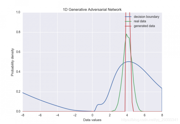
这很直观。 鉴别器正在查看来自真实数据和来自我们的发生器的各个样本。如果在这个简单的例子中，生成器只是产生实际数据的平均值，那么就很可能愚弄鉴别器。

这个问题有很多可能的解决方案。 在这种情况下，我们可以添加某种早期停止标准，当两个分布之间的相似度阈值达到时，暂停训练。 然而，如何把这个问题推广到更大的问题还不是很清楚，即使在简单的情况下，也很难保证我们的生成器分布总是会到达“有意义的早停”地步。 更有吸引力的解决方案是直接通过给予鉴别器一次检查多个例子的能力来解决问题。

Improving sample diversity

根据最近由Tim Salimans和OpenAI的合作者撰写的一篇论文，生成器输出非常窄的点分布是GAN的“主要失效模式之一”。值得庆幸的是，他们还提出了一个解决方案：允许鉴别者一次看多个样本，这种技术称为“小批量鉴别”（minibatch discrimination）。

在本文中，“小批量辨别”被定义为：鉴别器能够查看整批样品以决定它们是来自生成器还是来自真实数据。他们还提出了一个更具体的算法，该算法通过建模给定样本与同一批次中的所有其他样本之间的距离来工作。然后，这些距离与原始样本结合并通过鉴别器，因此它可以在分类过程中选择使用距离度量和样本值。

该方法可以粗略地总结如下：

• 取出鉴别器中间层的输出。

• 将其乘以三维张量以生成矩阵（在下面的代码中，大小为num_kernels x kernel_dim）。

• 计算一个批次中所有样本矩阵中行间的L1距离，然后应用负指数。

• 样本的minibatch特征是这些指数化距离的总和。

• 使用新创建的小块功能将原始输入连接到小批量图层（以前的鉴别图层的输出），并将其作为输入传递到鉴别器的下一层。

• 在TensorFlow中可以翻译成如下的东西：

    def minibatch(input, num_kernels=5, kernel_dim=3):
        x = linear(input, num_kernels * kernel_dim)
        activation = tf.reshape(x, (-1, num_kernels, kernel_dim))
        diffs = tf.expand_dims(activation, 3) -  tf.expand_dims(tf.transpose(activation, [1, 2, 0]), 0)
        abs_diffs = tf.reduce_sum(tf.abs(diffs), 2)
        minibatch_features = tf.reduce_sum(tf.exp(-abs_diffs), 2)
        return tf.concat(1, [input, minibatch_features])
  

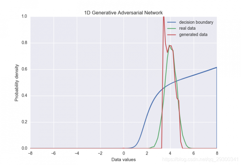
我们实现了提议的“小批量辨别”技术，看看它是否有助于解决我们例子中发生器输出分布的崩溃。下面显示了训练期间发生器网络的新行为。

在这种情况下很明显，添加小批量区分会使发生器保持原始数据分布的大部分宽度（尽管它还不完美）。 收敛之后，分布现在看起来像这样：

关于“小批量辨别”的最后一点是它使得批量的大小作为一个超参数变得更加重要。在我们的例子中，我们必须保持批量相当小（小于16左右）以便训练集中。也许只是限制每个距离度量的样本数量就足够了，而不是使用整个批次，但是这个又一个参数调整。

Final thoughts

生成对抗网络是一个有趣的发展，为我们提供了一种新的无监督学习方式。 GAN的大部分成功应用都在计算机视觉领域，但在这里，我们正在研究如何将这些技术应用于自然语言处理。

这方面的一个大问题就是如何最好地评估这些模型。在图像领域，至少看看生成的样本是相当容易的，尽管这显然不是一个令人满意的解决方案。在文本领域，这一点甚至没有用处（除非你的目标是产生散文）。对于基于最大似然训练的生成模型，我们通常可以基于未知的测试数据的可能性（或者可能性的一些下限）产生一些度量，但是这不适用于此。一些GAN论文已经根据生成的样本的核密度估计产生了似然估计，但是这种技术似乎在高维空间中被破坏了。另一个解决方案是只评估一些下游任务（如分类）。

最后是完整代码

'''
An example of distribution approximation using Generative Adversarial Networks
in TensorFlow.

Based on the blog post by Eric Jang:
http://blog.evjang.com/2016/06/generative-adversarial-nets-in.html,

and of course the original GAN paper by Ian Goodfellow et. al.:
https://arxiv.org/abs/1406.2661.

The minibatch discrimination technique is taken from Tim Salimans et. al.:
https://arxiv.org/abs/1606.03498.
'''

import argparse
import numpy as np
import tensorflow as tf
import matplotlib.pyplot as plt
from matplotlib import animation
import seaborn as sns

sns.set(color_codes=True)

seed = 42
np.random.seed(seed)
tf.set_random_seed(seed)


class DataDistribution(object):
    def __init__(self):
        self.mu = 4
        self.sigma = 0.5

    def sample(self, N):
        samples = np.random.normal(self.mu, self.sigma, N)
        samples.sort()
        return samples


class GeneratorDistribution(object):
    def __init__(self, range):
        self.range = range

    def sample(self, N):
        return np.linspace(-self.range, self.range, N) + \
            np.random.random(N) * 0.01


def linear(input, output_dim, scope=None, stddev=1.0):
    with tf.variable_scope(scope or 'linear'):
        w = tf.get_variable(
            'w',
            [input.get_shape()[1], output_dim],
            initializer=tf.random_normal_initializer(stddev=stddev)
        )
        b = tf.get_variable(
            'b',
            [output_dim],
            initializer=tf.constant_initializer(0.0)
        )
        return tf.matmul(input, w) + b


def generator(input, h_dim):
    h0 = tf.nn.softplus(linear(input, h_dim, 'g0'))
    h1 = linear(h0, 1, 'g1')
    return h1


def discriminator(input, h_dim, minibatch_layer=True):
    h0 = tf.nn.relu(linear(input, h_dim * 2, 'd0'))
    h1 = tf.nn.relu(linear(h0, h_dim * 2, 'd1'))

    # without the minibatch layer, the discriminator needs an additional layer
    # to have enough capacity to separate the two distributions correctly
    if minibatch_layer:
        h2 = minibatch(h1)
    else:
        h2 = tf.nn.relu(linear(h1, h_dim * 2, scope='d2'))

    h3 = tf.sigmoid(linear(h2, 1, scope='d3'))
    return h3


def minibatch(input, num_kernels=5, kernel_dim=3):
    x = linear(input, num_kernels * kernel_dim, scope='minibatch', stddev=0.02)
    activation = tf.reshape(x, (-1, num_kernels, kernel_dim))
    diffs = tf.expand_dims(activation, 3) - \
        tf.expand_dims(tf.transpose(activation, [1, 2, 0]), 0)
    abs_diffs = tf.reduce_sum(tf.abs(diffs), 2)
    minibatch_features = tf.reduce_sum(tf.exp(-abs_diffs), 2)
    return tf.concat([input, minibatch_features], 1)


def optimizer(loss, var_list):
    learning_rate = 0.001
    step = tf.Variable(0, trainable=False)
    optimizer = tf.train.AdamOptimizer(learning_rate).minimize(
        loss,
        global_step=step,
        var_list=var_list
    )
    return optimizer


def log(x):
    '''
    Sometimes discriminiator outputs can reach values close to
    (or even slightly less than) zero due to numerical rounding.
    This just makes sure that we exclude those values so that we don't
    end up with NaNs during optimisation.
    '''
    return tf.log(tf.maximum(x, 1e-5))


class GAN(object):
    def __init__(self, params):
        # This defines the generator network - it takes samples from a noise
        # distribution as input, and passes them through an MLP.
        with tf.variable_scope('G'):
            self.z = tf.placeholder(tf.float32, shape=(params.batch_size, 1))
            self.G = generator(self.z, params.hidden_size)

        # The discriminator tries to tell the difference between samples from
        # the true data distribution (self.x) and the generated samples
        # (self.z).
        #
        # Here we create two copies of the discriminator network
        # that share parameters, as you cannot use the same network with
        # different inputs in TensorFlow.
        self.x = tf.placeholder(tf.float32, shape=(params.batch_size, 1))
        with tf.variable_scope('D'):
            self.D1 = discriminator(
                self.x,
                params.hidden_size,
                params.minibatch
            )
        with tf.variable_scope('D', reuse=True):
            self.D2 = discriminator(
                self.G,
                params.hidden_size,
                params.minibatch
            )

        # Define the loss for discriminator and generator networks
        # (see the original paper for details), and create optimizers for both
        self.loss_d = tf.reduce_mean(-log(self.D1) - log(1 - self.D2))
        self.loss_g = tf.reduce_mean(-log(self.D2))

        vars = tf.trainable_variables()
        self.d_params = [v for v in vars if v.name.startswith('D/')]
        self.g_params = [v for v in vars if v.name.startswith('G/')]

        self.opt_d = optimizer(self.loss_d, self.d_params)
        self.opt_g = optimizer(self.loss_g, self.g_params)


def train(model, data, gen, params):
    anim_frames = []

    with tf.Session() as session:
        tf.local_variables_initializer().run()
        tf.global_variables_initializer().run()

        for step in range(params.num_steps + 1):
            # update discriminator
            x = data.sample(params.batch_size)
            z = gen.sample(params.batch_size)
            loss_d, _, = session.run([model.loss_d, model.opt_d], {
                model.x: np.reshape(x, (params.batch_size, 1)),
                model.z: np.reshape(z, (params.batch_size, 1))
            })

            # update generator
            z = gen.sample(params.batch_size)
            loss_g, _ = session.run([model.loss_g, model.opt_g], {
                model.z: np.reshape(z, (params.batch_size, 1))
            })

            if step % params.log_every == 0:
                print('{}: {:.4f}\t{:.4f}'.format(step, loss_d, loss_g))

            if params.anim_path and (step % params.anim_every == 0):
                anim_frames.append(
                    samples(model, session, data, gen.range, params.batch_size)
                )

        if params.anim_path:
            save_animation(anim_frames, params.anim_path, gen.range)
        else:
            samps = samples(model, session, data, gen.range, params.batch_size)
            plot_distributions(samps, gen.range)


def samples(
    model,
    session,
    data,
    sample_range,
    batch_size,
    num_points=10000,
    num_bins=100
):
    '''
    Return a tuple (db, pd, pg), where db is the current decision
    boundary, pd is a histogram of samples from the data distribution,
    and pg is a histogram of generated samples.
    '''
    xs = np.linspace(-sample_range, sample_range, num_points)
    bins = np.linspace(-sample_range, sample_range, num_bins)

    # decision boundary
    db = np.zeros((num_points, 1))
    for i in range(num_points // batch_size):
        db[batch_size * i:batch_size * (i + 1)] = session.run(
            model.D1,
            {
                model.x: np.reshape(
                    xs[batch_size * i:batch_size * (i + 1)],
                    (batch_size, 1)
                )
            }
        )

    # data distribution
    d = data.sample(num_points)
    pd, _ = np.histogram(d, bins=bins, density=True)

    # generated samples
    zs = np.linspace(-sample_range, sample_range, num_points)
    g = np.zeros((num_points, 1))
    for i in range(num_points // batch_size):
        g[batch_size * i:batch_size * (i + 1)] = session.run(
            model.G,
            {
                model.z: np.reshape(
                    zs[batch_size * i:batch_size * (i + 1)],
                    (batch_size, 1)
                )
            }
        )
    pg, _ = np.histogram(g, bins=bins, density=True)

    return db, pd, pg


def plot_distributions(samps, sample_range):
    db, pd, pg = samps
    db_x = np.linspace(-sample_range, sample_range, len(db))
    p_x = np.linspace(-sample_range, sample_range, len(pd))
    f, ax = plt.subplots(1)
    ax.plot(db_x, db, label='decision boundary')
    ax.set_ylim(0, 1)
    plt.plot(p_x, pd, label='real data')
    plt.plot(p_x, pg, label='generated data')
    plt.title('1D Generative Adversarial Network')
    plt.xlabel('Data values')
    plt.ylabel('Probability density')
    plt.legend()
    plt.show()


def save_animation(anim_frames, anim_path, sample_range):
    f, ax = plt.subplots(figsize=(6, 4))
    f.suptitle('1D Generative Adversarial Network', fontsize=15)
    plt.xlabel('Data values')
    plt.ylabel('Probability density')
    ax.set_xlim(-6, 6)
    ax.set_ylim(0, 1.4)
    line_db, = ax.plot([], [], label='decision boundary')
    line_pd, = ax.plot([], [], label='real data')
    line_pg, = ax.plot([], [], label='generated data')
    frame_number = ax.text(
        0.02,
        0.95,
        '',
        horizontalalignment='left',
        verticalalignment='top',
        transform=ax.transAxes
    )
    ax.legend()

    db, pd, _ = anim_frames[0]
    db_x = np.linspace(-sample_range, sample_range, len(db))
    p_x = np.linspace(-sample_range, sample_range, len(pd))

    def init():
        line_db.set_data([], [])
        line_pd.set_data([], [])
        line_pg.set_data([], [])
        frame_number.set_text('')
        return (line_db, line_pd, line_pg, frame_number)

    def animate(i):
        frame_number.set_text(
            'Frame: {}/{}'.format(i, len(anim_frames))
        )
        db, pd, pg = anim_frames[i]
        line_db.set_data(db_x, db)
        line_pd.set_data(p_x, pd)
        line_pg.set_data(p_x, pg)
        return (line_db, line_pd, line_pg, frame_number)

    anim = animation.FuncAnimation(
        f,
        animate,
        init_func=init,
        frames=len(anim_frames),
        blit=True
    )
    anim.save(anim_path, fps=30, extra_args=['-vcodec', 'libx264'])


def main(args):
    model = GAN(args)
    train(model, DataDistribution(), GeneratorDistribution(range=8), args)


def parse_args():
    parser = argparse.ArgumentParser()
    parser.add_argument('--num-steps', type=int, default=5000,
                        help='the number of training steps to take')
    parser.add_argument('--hidden-size', type=int, default=4,
                        help='MLP hidden size')
    parser.add_argument('--batch-size', type=int, default=8,
                        help='the batch size')
    parser.add_argument('--minibatch', action='store_true',
                        help='use minibatch discrimination')
    parser.add_argument('--log-every', type=int, default=10,
                        help='print loss after this many steps')
    parser.add_argument('--anim-path', type=str, default=None,
                        help='path to the output animation file')
    parser.add_argument('--anim-every', type=int, default=1,
                        help='save every Nth frame for animation')
    return parser.parse_args()


if __name__ == '__main__':
    main(parse_args())

代码说明：

An introduction to Generative Adversarial Networks

This is the code that we used to generate our GAN 1D Gaussian approximation.
For more information see our blog post: http://blog.aylien.com/introduction-generative-adversarial-networks-code-tensorflow.

Installing dependencies

Written for Python 3.x (tested on 3.6.1).

For the Python dependencies, first install the requirements file:

$ pip install -r requirements.txt

If you want to also generate the animations, you need to also make sure that ffmpeg is installed and on your path.

Training

For a full list of parameters, run:

$ python gan.py --help

To run without minibatch discrimination (and plot the resulting distributions):

$ python gan.py

To run with minibatch discrimination (and plot the resulting distributions):

$ python gan.py --minibatch

requirements.txt文件

matplotlib==1.5.3
numpy==1.11.3
scipy==0.17.0
seaborn==0.7.1
tensorflow==1.2.0

运行前需要安装
sudo apt-get install python3-tk