LM解非线性最小二乘--以圆锥面拟合为例

圆锥面方程

此处我们将模型简化为一个中心轴始终与z轴平行的圆锥面，该圆锥面包括4个参数，分别为锥点坐标（a, b, c）和半顶角α。

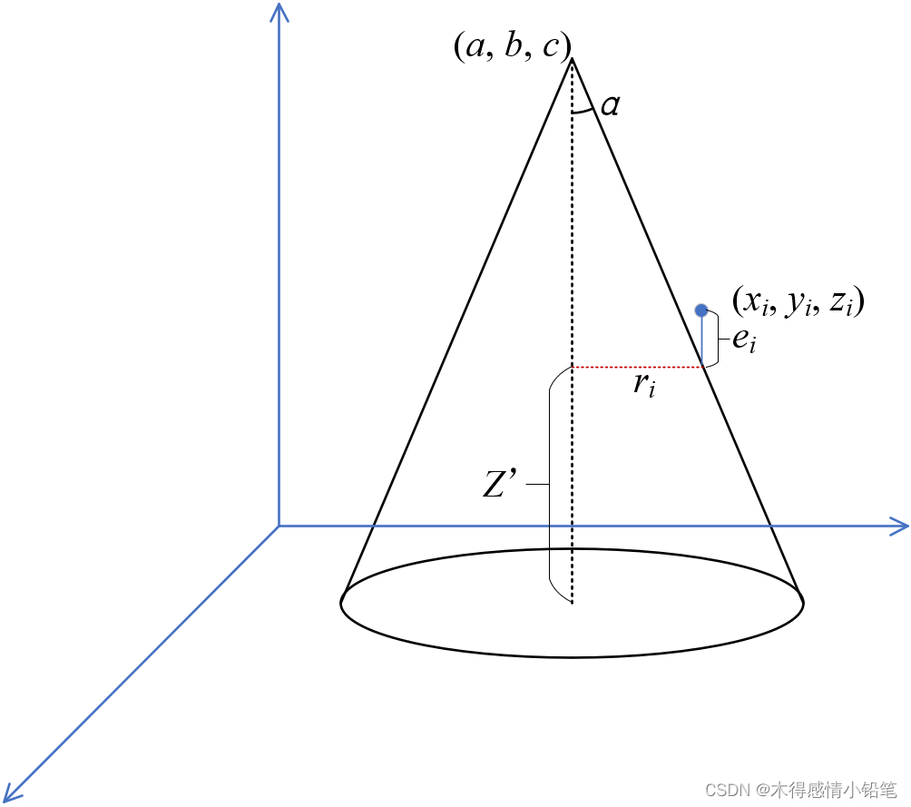
则圆锥面上一点对应的高程z’可表达为：
$$z=c-\sqrt{{\left(x-a\right)}^2+{\left(y-b\right)}^2}\times \frac{1}{\tan \alpha }.$$

LM解非线性最小二乘

根据圆锥面方程，我们可以定义误差方程为：
$$r_i=z_i-c+\sqrt{{\left(x_i-a\right)}^2+{\left(y_i-b\right)}^2}\times \frac{1}{\tan \alpha }$$
显然这个误差方程是非线性的，要解这个方程有多种现成的方法，比如高斯牛顿法，Levenberg-Marquardt （LM）法等，这里我们采用最常用的LM法。

C++编程实现

第三方库：eigen

template<typename _Scalar, int NX = Eigen::Dynamic, int NY = Eigen::Dynamic>
struct Functor
{
	typedef _Scalar Scalar;
	enum {
		InputsAtCompileTime = NX,
		ValuesAtCompileTime = NY
	};
	typedef Eigen::Matrix<Scalar, InputsAtCompileTime, 1> InputType;
	typedef Eigen::Matrix<Scalar, ValuesAtCompileTime, 1> ValueType;
	typedef Eigen::Matrix<Scalar, ValuesAtCompileTime, InputsAtCompileTime> JacobianType;

	int m_inputs, m_values;

	Functor() : m_inputs(InputsAtCompileTime), m_values(ValuesAtCompileTime) {}
	Functor(int inputs, int values) : m_inputs(inputs), m_values(values) {}

	int inputs() const { return m_inputs; }
	int values() const { return m_values; }

};

//构建LM函数
struct LMFunctor : Functor<float> {
private:
	std::vector<Vec3>   mVec; // Data points to fit.
	int                 mSize; // Number of data points, i.e. values.

public:
	// Set the number of data points
	void setValues(std::vector<Vec3> vec)
	{
		mVec = vec;
		mSize = vec.size();
	}

	// Compute 'm' errors, one for each data point, for the given parameter values in 'x'
	int operator()(const Eigen::VectorXf& x, Eigen::VectorXf& fvec) const
	{
		// 'x' has dimensions n x 1
	    // It contains the current estimates for the parameters.

	    // 'fvec' has dimensions m x 1
	    // It will contain the error for each data point.

		float a = x(0);
		float b = x(1);
		float c = x(2);
		float d = x(3);

		for (int i = 0; i < values(); i++) {
			float x = mVec[i].f[0];
			float y = mVec[i].f[1];
			float z = mVec[i].f[2];

			fvec(i) = z - c + std::sqrt((x - a) * (x - a) + (y - b) * (y - b)) / std::tan(d);
		}

		return 0;
	}

	// Compute the jacobian of the errors
	int df(const Eigen::VectorXf& x, Eigen::MatrixXf& fjac) const
	{
		// 'x' has dimensions n x 1
        // It contains the current estimates for the parameters.

        // 'fjac' has dimensions m x n
        // It will contain the jacobian of the errors, calculated numerically in this case.

		float epsilon;
		epsilon = 1e-5f;

		for (int i = 0; i < x.size(); i++) {
			Eigen::VectorXf xPlus(x);
			xPlus(i) += epsilon;
			Eigen::VectorXf xMinus(x);
			xMinus(i) -= epsilon;

			Eigen::VectorXf fvecPlus(values());
			operator()(xPlus, fvecPlus);

			Eigen::VectorXf fvecMinus(values());
			operator()(xMinus, fvecMinus);

			Eigen::VectorXf fvecDiff(values());
			fvecDiff = (fvecPlus - fvecMinus) / (2.0f * epsilon);

			fjac.block(0, i, values(), 1) = fvecDiff;
		}

		return 0;
	}

	// Returns 'mSize', the number of values.
	int values() const { return mSize; }
};

其中jacobian矩阵的计算可以使用手动求导方法，也可以采用我给出的有限差分方法，如果对自己算的对不对没信心的话还是老实拷贝代码吧。
最后就是采用LM解方程了：

	// 圆锥曲面的方程参数，表示为 (x0,y0,z0,alpha)
	Eigen::VectorXf params = Eigen::VectorXf(4, 1);

	LMFunctor functor;
	functor.setValues(cloud); //cloud为待拟合数据
	Eigen::NumericalDiff<LMFunctor> numDiff(functor);
	Eigen::LevenbergMarquardt<Eigen::NumericalDiff<LMFunctor>, float> lm(numDiff);
	lm.parameters.maxfev = 1000;
	lm.parameters.xtol = 1.0e-10;
	int ret = lm.minimize(params);
	
	// 输出最优拟合参数
	std::cout << "The optimal parameters are: " << params.transpose() << std::endl;

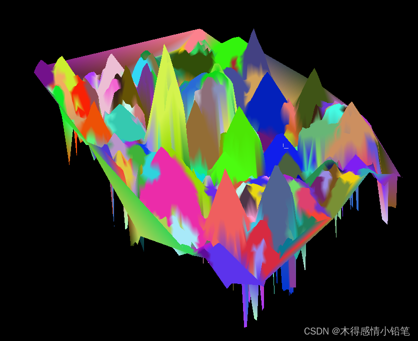
至此圆锥面拟合完成：