


前言
K-Center-Greedy 算法在主动学习和数据采样、最大覆盖等方面有广泛的应用。
最主要的思想是,可以用k个中心点来代表目前的数据分布。
算法流程
初始化:随机选择一个sample作为第一个中心。
计算数据集中每个sample到中心点的距离,并找出每个sample到中心点最小的距离,即计算数据集中每个点到其最近中心点的距离,我们称之为每个点的最近中心点距离。
选择目前所有样本点中的最近中心点距离最大的那个作为新的中心点。(即距离现有中心点最远的那个样本作为新的中心点)
重复2-3, 直到选择出k个中心点
其实可以简单一句话总结(上面的表述有点子绕 可能),这个算法的中心思想:就是找出目前样本中和目前所有中心点最远的那个点,作为新的中心点。
简单实现
import numpy as np
from scipy.spatial import distance
import matplotlib.pyplot as plt


def k_center_greedy(X, k):
    # 随机选择第一个中心点
    centers = [X[np.random.choice(range(X.shape[0]))]]

    while len(centers) < k:
        # 计算数据集中每个点到其最近中心点的最小距离
        dist_to_closest_center = np.array([min([distance.euclidean(x, c) for c in centers]) for x in X])

        # 选择距离现有中心点最远的点
        new_center = X[np.argmax(dist_to_closest_center)]
        centers.append(new_center)

    return np.array(centers)


def plot_k_center_greedy(points, centers):
    plt.scatter(points[:, 0], points[:, 1], c='blue', label='Data Points')
    plt.scatter(centers[:, 0], centers[:, 1], c='red', marker='x', s=100, label='Center Points')
    plt.title('K-Center-Greedy Result')
    plt.xlabel('Dimension 1')
    plt.ylabel('Dimension 2')
    plt.legend()
    plt.show()


if __name__ == '__main__':
    points = np.random.rand(200, 2) * 100
    k = 10
    centers = k_center_greedy(points, k)
    plot_k_center_greedy(points, centers)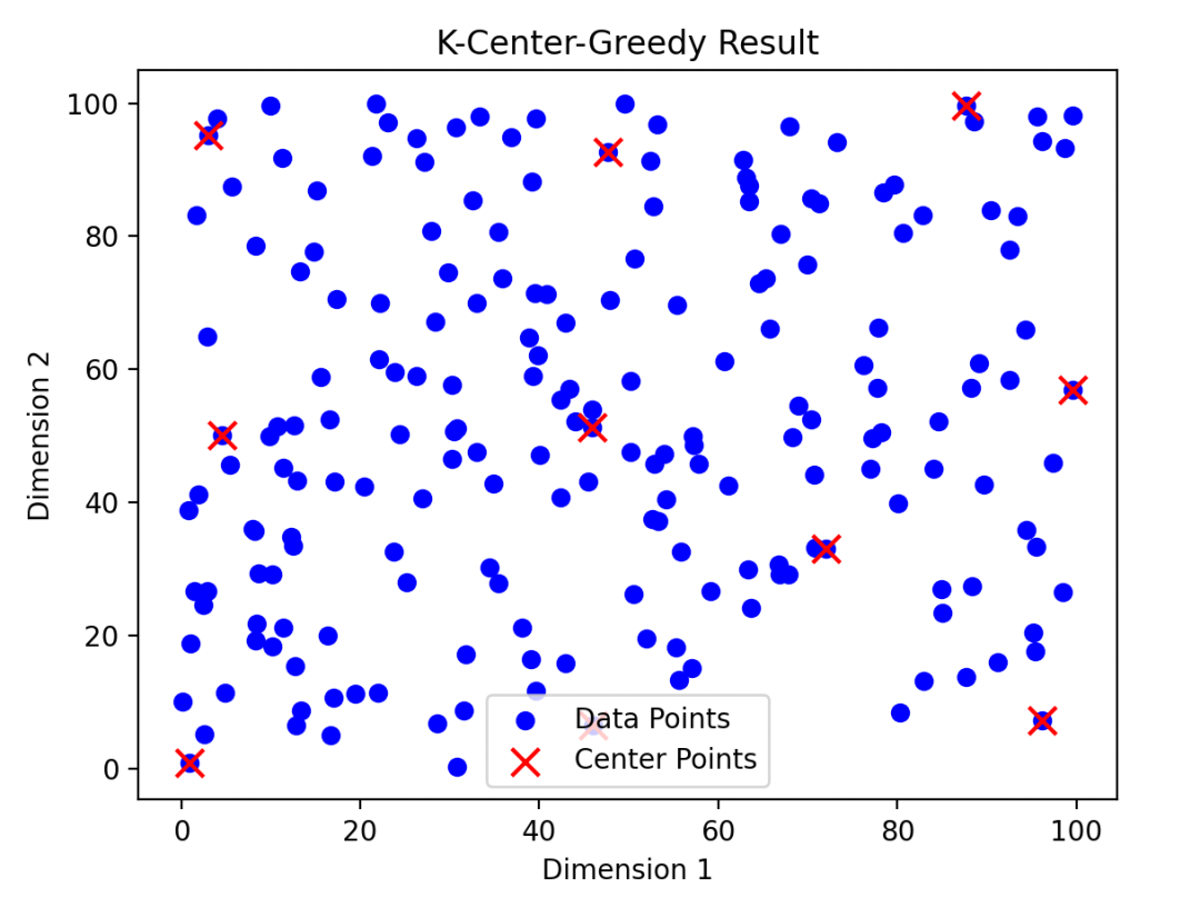
更节省空间,更结构化的实现
import numpy as np
from sklearn.metrics.pairwise import cosine_distances, euclidean_distances
import matplotlib.pyplot as plt


def cal_distance(x, y, mod="euc"):
    if mod == "cos":
        distance = cosine_distances(X=x.reshape(1, -1),
                                    Y=y.reshape(1, -1))  # 与簇的质心的最小距离
        distance = distance[0][0]
        return distance
    elif mod == "euc":
        distance = euclidean_distances(X=x.reshape(1, -1),
                                       Y=y.reshape(1, -1))
        distance = distance[0][0]
        return distance


class KCenterGreedy:
    def __init__(self, k):
        self.k = k
        self.centers = []
        self.select_index_list = []

    def fit(self, data):
        self.centers = []
        init_index = np.random.choice(range(data.shape[0]))
        self.centers.append(init_index)

        while len(self.centers) < self.k:
            # 计算数据集中每个点到其最近中心点的最小距离
            dist_to_closest_center = np.array(
                [min([cal_distance(x, data[c]) for c in self.centers]) for index, x in enumerate(data)]
            )

            # 选择距离现有中心点最远的点
            new_index = np.argmax(dist_to_closest_center)
            self.centers.append(new_index)

    def get_center(self):
        return list(set(self.centers))

def plot_k_center_greedy(points, centers):
    plt.scatter(points[:, 0], points[:, 1], c='blue', label='Data Points')
    plt.scatter(centers[:, 0], centers[:, 1], c='red', marker='x', s=100, label='Center Points')
    plt.title('K-Center-Greedy Result')
    plt.xlabel('Dimension 1')
    plt.ylabel('Dimension 2')
    plt.legend()
    plt.show()


if __name__ == '__main__':
    np.random.seed(1996)
    points = np.random.rand(200, 2) * 100
    k = 20

    kc_greedy = KCenterGreedy(k)
    kc_greedy.fit(points)

    centers_index = kc_greedy.centers
    centers = points[centers_index]
    print("Center points:")
    print(kc_greedy.get_center(), len(kc_greedy.get_center()))
    # 绘制结果
    plot_k_center_greedy(points, centers)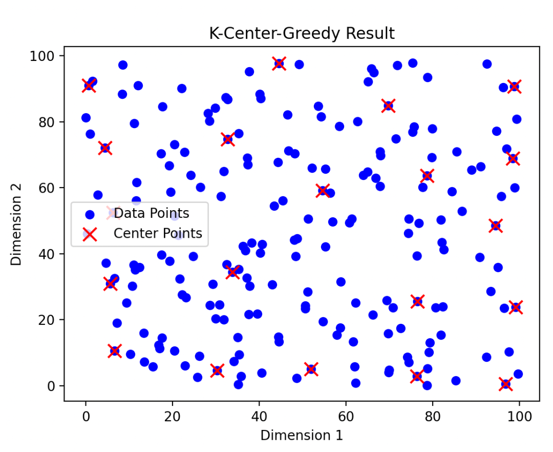
算法的优缺点
优点
适用于大规模数据
最大化数据多样性
缺点
计算复杂度较高
对噪声敏感
推荐阅读:
公众号:AI蜗牛车
保持谦逊、保持自律、保持进步

发送【蜗牛】获取一份《手把手AI项目》(AI蜗牛车著)
发送【1222】获取一份不错的leetcode刷题笔记
发送【AI四大名著】获取四本经典AI电子书


 2618
2618

 被折叠的 条评论
为什么被折叠?
被折叠的 条评论
为什么被折叠?
 到【灌水乐园】发言


