


目录
之前写过一次,这篇是再修改版本( 前版本)
1.观察并导入数据
import numpy as np
import pandas as pd
import matplotlib.pyplot as plt
plt.rcParams['font.sans-serif']=['SimHei'] #用来正常显示中文标签
plt.rcParams['axes.unicode_minus'] = False #用来正常显示负号
df = pd.read_csv('adults.csv')
df.info()
<class 'pandas.core.frame.DataFrame'>
RangeIndex: 32561 entries, 0 to 32560
Data columns (total 15 columns):
 #   Column          Non-Null Count  Dtype
---  ------          --------------  -----
 0   age             32561 non-null  int64
 1   workclass       32561 non-null  object
 2   final_weight    32561 non-null  int64
 3   education       32561 non-null  object
 4   education_num   32561 non-null  int64
 5   marital_status  32561 non-null  object
 6   occupation      32561 non-null  object
 7   relationship    32561 non-null  object
 8   race            32561 non-null  object
 9   sex             32561 non-null  object
 10  capital_gain    32561 non-null  int64
 11  capital_loss    32561 non-null  int64
 12  hours_per_week  32561 non-null  int64
 13  native_country  32561 non-null  object
 14  salary          32561 non-null  object
dtypes: int64(6), object(9)
memory usage: 3.7+ MB
df.head()
| age | workclass | final_weight | education | education_num | marital_status | occupation | relationship | race | sex | capital_gain | capital_loss | hours_per_week | native_country | salary | |
|---|---|---|---|---|---|---|---|---|---|---|---|---|---|---|---|
| 0 | 39 | State-gov | 77516 | Bachelors | 13 | Never-married | Adm-clerical | Not-in-family | White | Male | 2174 | 0 | 40 | United-States | <=50K |
| 1 | 50 | Self-emp-not-inc | 83311 | Bachelors | 13 | Married-civ-spouse | Exec-managerial | Husband | White | Male | 0 | 0 | 13 | United-States | <=50K |
| 2 | 38 | Private | 215646 | HS-grad | 9 | Divorced | Handlers-cleaners | Not-in-family | White | Male | 0 | 0 | 40 | United-States | <=50K |
| 3 | 53 | Private | 234721 | 11th | 7 | Married-civ-spouse | Handlers-cleaners | Husband | Black | Male | 0 | 0 | 40 | United-States | <=50K |
| 4 | 28 | Private | 338409 | Bachelors | 13 | Married-civ-spouse | Prof-specialty | Wife | Black | Female | 0 | 0 | 40 | Cuba | <=50K |
df.workclass.value_counts()
Private             22696
Self-emp-not-inc     2541
Local-gov            2093
?                    1836
State-gov            1298
Self-emp-inc         1116
Federal-gov           960
Without-pay            14
Never-worked            7
Name: workclass, dtype: int64
df.capital_gain.value_counts()
0        29849
15024      347
7688       284
7298       246
99999      159
         ...
1111         1
2538         1
22040        1
4931         1
5060         1
Name: capital_gain, Length: 119, dtype: int64
df.salary.value_counts()
<=50K    24720
>50K      7841
Name: salary, dtype: int64
# 过采样 重复少的/收集新的/算法伪造
# 欠采样 抛弃多的数据
#
2. 处理数据
缺失值处理
# 缺失值都是用  ? 替换的
df = df.replace('?',np.nan)
df.info()
<class 'pandas.core.frame.DataFrame'>
RangeIndex: 32561 entries, 0 to 32560
Data columns (total 15 columns):
 #   Column          Non-Null Count  Dtype
---  ------          --------------  -----
 0   age             32561 non-null  int64
 1   workclass       30725 non-null  object
 2   final_weight    32561 non-null  int64
 3   education       32561 non-null  object
 4   education_num   32561 non-null  int64
 5   marital_status  32561 non-null  object
 6   occupation      30718 non-null  object
 7   relationship    32561 non-null  object
 8   race            32561 non-null  object
 9   sex             32561 non-null  object
 10  capital_gain    32561 non-null  int64
 11  capital_loss    32561 non-null  int64
 12  hours_per_week  32561 non-null  int64
 13  native_country  31978 non-null  object
 14  salary          32561 non-null  object
dtypes: int64(6), object(9)
memory usage: 3.7+ MB
2.1探索数据(对df进行数据探索,df为将’?’ 替换为np.nan 的数据集,clean_df 为删除了’?'所在行的数据集)
import seaborn as sns
%matplotlib inline
#检查数据相关性
sns.heatmap(df.corr()
           ,annot=True
           ,center=0
           ,linewidth=0.8)
<AxesSubplot:>
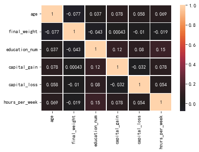
直接检查相关性似乎并不妥当,因为数据并不都是数值类型
查看数值类型的特征:
df.describe([0.01,0.99]).T
| count | mean | std | min | 1% | 50% | 99% | max | |
|---|---|---|---|---|---|---|---|---|
| age | 32561.0 | 38.581647 | 13.640433 | 17.0 | 17.0 | 37.0 | 74.0 | 90.0 |
| final_weight | 32561.0 | 189778.366512 | 105549.977697 | 12285.0 | 27185.8 | 178356.0 | 510072.0 | 1484705.0 |
| education_num | 32561.0 | 10.080679 | 2.572720 | 1.0 | 3.0 | 10.0 | 16.0 | 16.0 |
| capital_gain | 32561.0 | 1077.648844 | 7385.292085 | 0.0 | 0.0 | 0.0 | 15024.0 | 99999.0 |
| capital_loss | 32561.0 | 87.303830 | 402.960219 | 0.0 | 0.0 | 0.0 | 1980.0 | 4356.0 |
| hours_per_week | 32561.0 | 40.437456 | 12.347429 | 1.0 | 8.0 | 40.0 | 80.0 | 99.0 |
df.describe([0.01,0.99]).T.index
Index(['age', 'final_weight', 'education_num', 'capital_gain', 'capital_loss',
       'hours_per_week'],
      dtype='object')
# 年龄分布
sns.set_style('whitegrid')
plt.subplots(figsize=(15,8))
s = df['age'].value_counts()
sns.barplot(s.index,s.values)
<AxesSubplot:>
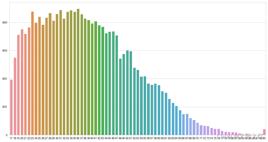
df.age.mean() # 平均年龄
38.58164675532078
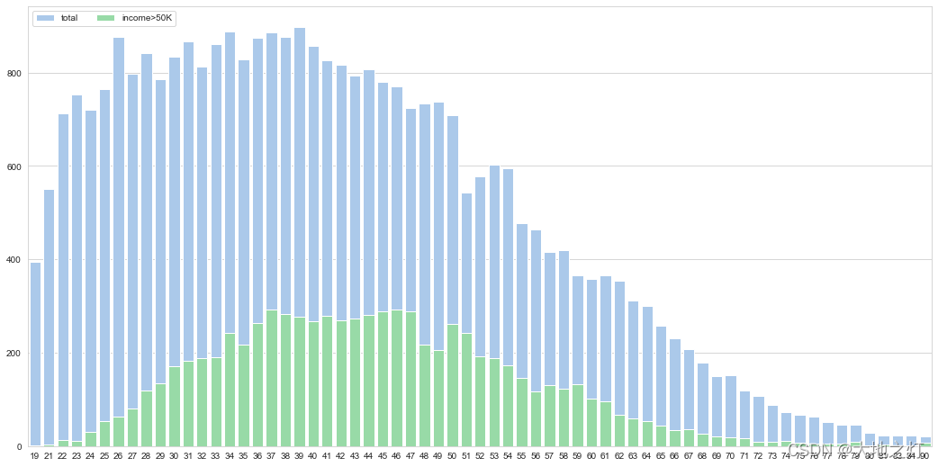
# 第一,年龄和工资的关系
s=df['age'].value_counts()
k=df['age'][df['salary']=='>50K'].value_counts()
sns.set_style("whitegrid")
f, ax = plt.subplots(figsize=(18, 9))
sns.set_color_codes("pastel")
sns.barplot(s.index,s.values,label='total',color="b")
sns.barplot(k.index,k.values,label='income>50K',color="g")
ax.legend(ncol=2, loc="upper left", frameon=True)
<matplotlib.legend.Legend at 0x16cd08a8be0>
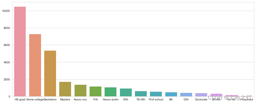
# 第二,教育水平
# 高中毕业人数有将近1.6万人,其次是大学肄业
plt.subplots(figsize=(15,6))
s = df['education'].value_counts()
sns.barplot(s.index,s.values)
<AxesSubplot:>
df['education_num'].value_counts()
9     10501
10     7291
13     5355
14     1723
11     1382
7      1175
12     1067
6       933
4       646
15      576
5       514
8       433
16      413
3       333
2       168
1        51
Name: education_num, dtype: int64
edu_n = df.groupby(['education','education_num'])['education'].count()
edu_n
education     education_num
10th          6                  933
11th          7                 1175
12th          8                  433
1st-4th       2                  168
5th-6th       3                  333
7th-8th       4                  646
9th           5                  514
Assoc-acdm    12                1067
Assoc-voc     11                1382
Bachelors     13                5355
Doctorate     16                 413
HS-grad       9                10501
Masters       14                1723
Preschool     1                   51
Prof-school   15                 576
Some-college  10                7291
Name: education, dtype: int64
education 和 educational-num 是一一对应关系,做算法模型时可以删除一列。
education是分类变量,educational-num是数值变量,受教育水平是有顺序的,数字大小是有比较意义的,因此保留education-num。
s
HS-grad         10501
Some-college     7291
Bachelors        5355
Masters          1723
Assoc-voc        1382
11th             1175
Assoc-acdm       1067
10th              933
7th-8th           646
Prof-school       576
9th               514
12th              433
Doctorate         413
5th-6th           333
1st-4th           168
Preschool          51
Name: education, dtype: int64
edu_hsalary = df['education'][df['salary']=='>50K'].value_counts()
edu_lsalary = df['education'][df['salary']=='<=50K'].value_counts()

edu_high_percent = edu_hsalary/s
edu_low_percent = edu_lsalary/s

fig = plt.figure(figsize=(15,6))
sns.barplot(edu_high_percent.index,edu_high_percent.values,color='red',label='edu_high_salary')
sns.barplot(edu_low_percent.index,edu_low_percent.values,bottom = edu_high_percent,color='yellow',label='edu_low_salary')

fig.legend(ncol=2,loc='upper center',frameon=True)
<matplotlib.legend.Legend at 0x16cd4147d30>
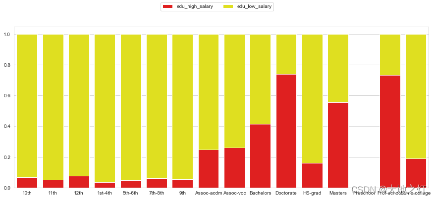
可以看到超过50K占比最高依次是,Prof-school,Doctorate,Masters,Bachelors 跟学习年限呈现正相关性。
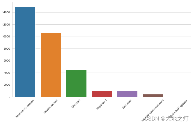
# 第三,婚姻状况
f,ax = plt.subplots(figsize=(11,6))
s=df['marital_status'].value_counts()
sns.barplot(s.index,s.values)
ax.set_xticklabels(ax.get_xticklabels(),rotation=45)
[Text(0, 0, 'Married-civ-spouse'),
 Text(1, 0, 'Never-married'),
 Text(2, 0, 'Divorced'),
 Text(3, 0, 'Separated'),
 Text(4, 0, 'Widowed'),
 Text(5, 0, 'Married-spouse-absent'),
 Text(6, 0, 'Married-AF-spouse')]
mer_hsalary=df['marital_status'][df['salary']=='>50K'].value_counts()
mer_lsalary=df['marital_status'][df['salary']=='<=50K'].value_counts()

f,ax = plt.subplots(figsize=[12,6])

sns.barplot(mer_hsalary.index,mer_hsalary.values,color='blue',alpha = 0.7,label='mer_low_salary')
sns.barplot(mer_lsalary.index,mer_lsalary.values,color='yellow',alpha = 0.5,label='mer_high_salary')

ax.legend(ncol=2,loc='upper center',frameon=True)
<matplotlib.legend.Legend at 0x16cd41a1b50>
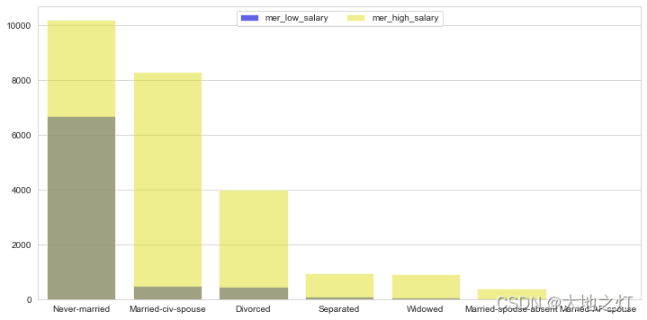
可以看到已婚和收入高低有正相关性,但还不能说明因此有因果关系。
# 第四、职业分布以及和收入关系
plt.subplots(figsize=(8,8))
s=df['occupation'].value_counts()
sns.barplot(y=s.index,x=s.values)
<AxesSubplot:>
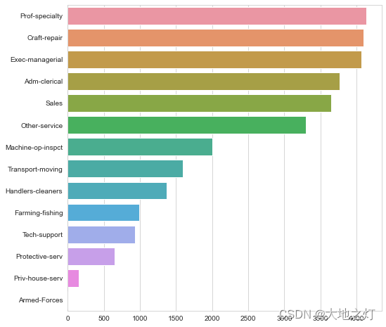
从业人数前三分别是Prof-specialty,Craft-repair,Exec-managerial
occ_hsalary=df['occupation'][df['salary']=='>50K'].value_counts()
occ_lsalary=df['occupation'][df['salary']=='<=50K'].value_counts()


f,ax=plt.subplots(figsize=[12,6])
a=s.index
sns.barplot(y=occ_hsalary.index,x=occ_hsalary.values,color='yellow',order=a,alpha = 0.7,label='occ_low_salary')

sns.barplot(y=occ_lsalary.index,x=occ_lsalary.values,color='blue',order=a,alpha=0.5,label='occ_high_salary')

ax.legend(ncol=2, loc="lower center", frameon=True)
<matplotlib.legend.Legend at 0x16cd4669100>
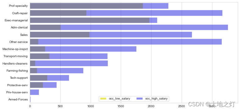
可以看出高收入占比比较高的是Exec-managerial、Prof-specialty,比较低的是Handlers-cleaners、Farming-fishing,比较符合我们的日常认知。
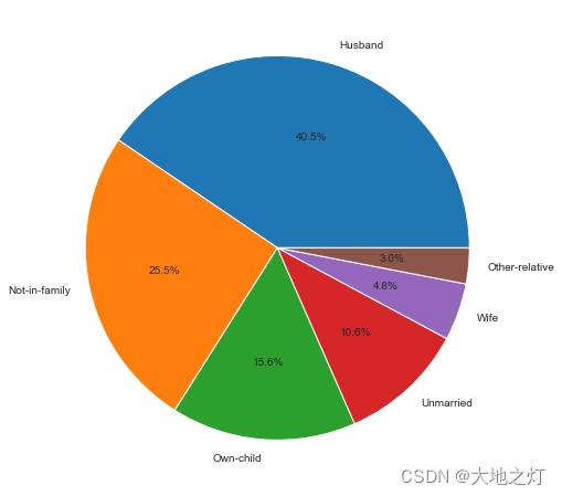
# 5 家庭
plt.subplots(figsize=(8,8))
s=df['relationship'].value_counts()
plt.pie(s.values,labels=s.index,autopct='%1.1f%%')
([<matplotlib.patches.Wedge at 0x16cd4114910>,
  <matplotlib.patches.Wedge at 0x16cd4119580>,
  <matplotlib.patches.Wedge at 0x16cd411f550>,
  <matplotlib.patches.Wedge at 0x16cd4126070>,
  <matplotlib.patches.Wedge at 0x16cd4126fd0>,
  <matplotlib.patches.Wedge at 0x16cd412bac0>],
 [Text(0.3228564400293403, 1.0515530034817937, 'Husband'),
  Text(-1.0768528506930521, -0.22447257728784475, 'Not-in-family'),
  Text(-0.08243982298868217, -1.0969064114980798, 'Own-child'),
  Text(0.7469351484545255, -0.8075195873805269, 'Unmarried'),
  Text(1.0368150199444963, -0.3674433485824635, 'Wife'),
  Text(1.0950764363882008, -0.10395960016909805, 'Other-relative')],
 [Text(0.1761035127432765, 0.5735743655355238, '40.5%'),
  Text(-0.5873742821962102, -0.12243958761155167, '25.5%'),
  Text(-0.04496717617564482, -0.5983125880898617, '15.6%'),
  Text(0.40741917188428656, -0.4404652294802873, '10.6%'),
  Text(0.5655354654242707, -0.20042364468134374, '4.8%'),
  Text(0.5973144198481095, -0.05670523645587165, '3.0%')])
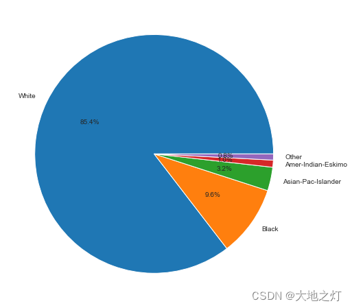
# 种族
plt.subplots(figsize=(8,8))
s=df['race'].value_counts()
plt.pie(s.values,labels=s.index,autopct='%1.1f%%')
([<matplotlib.patches.Wedge at 0x16cd4114a90>,
  <matplotlib.patches.Wedge at 0x16cd3f28550>,
  <matplotlib.patches.Wedge at 0x16cd3f28dc0>,
  <matplotlib.patches.Wedge at 0x16cd07c7d90>,
  <matplotlib.patches.Wedge at 0x16cd3e227c0>],
 [Text(-0.9867232454903924, 0.486186421868101, 'White'),
  Text(0.898950111132619, -0.6339469202501515, 'Black'),
  Text(1.0752451188481307, -0.23205157701095105, 'Asian-Pac-Islander'),
  Text(1.0962767570479313, -0.0904282696753132, 'Amer-Indian-Eskimo'),
  Text(1.0996240020243266, -0.028758549546243486, 'Other')],
 [Text(-0.5382126793583958, 0.2651925937462369, '85.4%'),
  Text(0.4903364242541558, -0.3457892292273554, '9.6%'),
  Text(0.5864973375535257, -0.12657358746051875, '3.2%'),
  Text(0.5979691402079624, -0.04932451073198901, '1.0%'),
  Text(0.5997949101950872, -0.015686481570678264, '0.8%')])
# 6 性别
df['sex'].value_counts()
Male      21790
Female    10771
Name: sex, dtype: int64
# 7 资本收益和损失
plt.subplots(figsize=(7,5))
sns.distplot(df['capital_loss'][df['capital_loss']!=0])
<AxesSubplot:xlabel='capital_loss', ylabel='Density'>
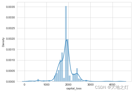
资本损失密度函数,峰值在2000左右,呈现正态分布
plt.subplots(figsize=(7,5))
sns.distplot(df['capital_gain'][df['capital_gain']!=0])
<AxesSubplot:xlabel='capital_gain', ylabel='Density'>
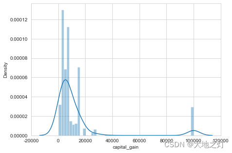
收益普遍比较高,在10万美金出现很多极值
df['capital_gain'][(df['capital_gain']!=0)|df['capital_loss']].agg(['mean','count'])
mean     8293.387852
count    4231.000000
Name: capital_gain, dtype: float64
df['capital_loss'][(df['capital_gain']!=0)|df['capital_loss']].agg(['mean','count'])
mean      671.874261
count    4231.000000
Name: capital_loss, dtype: float64
在有资本收益损失的调查人群6317人中,其中资本获益人均8343,资本损失人均676,看来行情不错。
gain_age=df.groupby(['age'])['capital_gain'].sum()
loss_age=df.groupby(['age'])['capital_loss'].sum()
fig =plt.figure(figsize=(15,6))
sns.barplot(gain_age.index,gain_age.values,color='yellow',alpha=0.7,label='capital_gain')
sns.barplot(loss_age.index,loss_age.values,color='red',alpha = 0.3,label='capital_loss')
fig.legend(ncol=2, loc="upper center", frameon=True)
<matplotlib.legend.Legend at 0x16cd3f471f0>
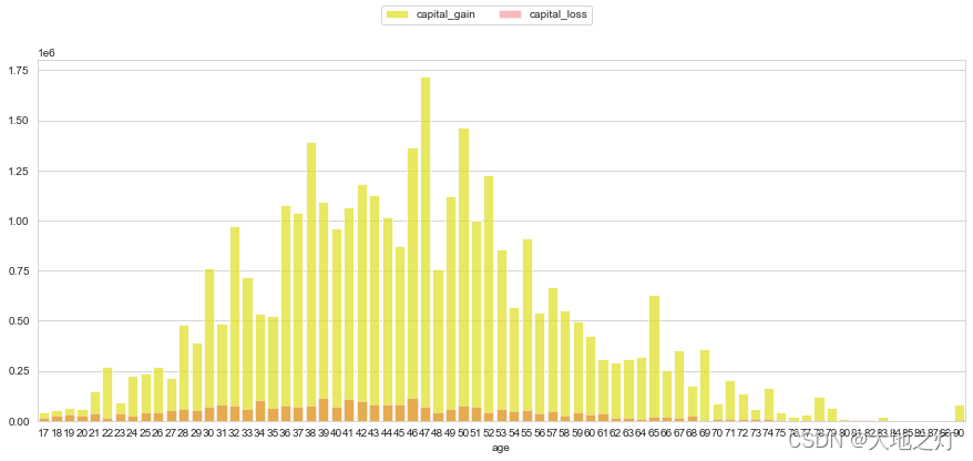
看下分年龄的资本收入情况对比。
# 8 工作时长
plt.subplots(figsize=(9,5))
sns.distplot(df['hours_per_week'])
<AxesSubplot:xlabel='hours_per_week', ylabel='Density'>
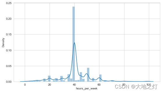
接近50%的人是每周工作40个小时。
plt.subplots(figsize=(8, 9))
s=df['native_country'][df['native_country']!='United-States'].value_counts()
sns.barplot(y=s.index,x=
            s.values)
<AxesSubplot:>

可以看到前三移民来源国是Mexico,Philippines,Germany
2.2缺失值情况分析
import missingno as msno # 可视化缺失值的库
df.info()
<class 'pandas.core.frame.DataFrame'>
RangeIndex: 32561 entries, 0 to 32560
Data columns (total 15 columns):
 #   Column          Non-Null Count  Dtype
---  ------          --------------  -----
 0   age             32561 non-null  int64
 1   workclass       30725 non-null  object
 2   final_weight    32561 non-null  int64
 3   education       32561 non-null  object
 4   education_num   32561 non-null  int64
 5   marital_status  32561 non-null  object
 6   occupation      30718 non-null  object
 7   relationship    32561 non-null  object
 8   race            32561 non-null  object
 9   sex             32561 non-null  object
 10  capital_gain    32561 non-null  int64
 11  capital_loss    32561 non-null  int64
 12  hours_per_week  32561 non-null  int64
 13  native_country  31978 non-null  object
 14  salary          32561 non-null  object
dtypes: int64(6), object(9)
memory usage: 3.7+ MB
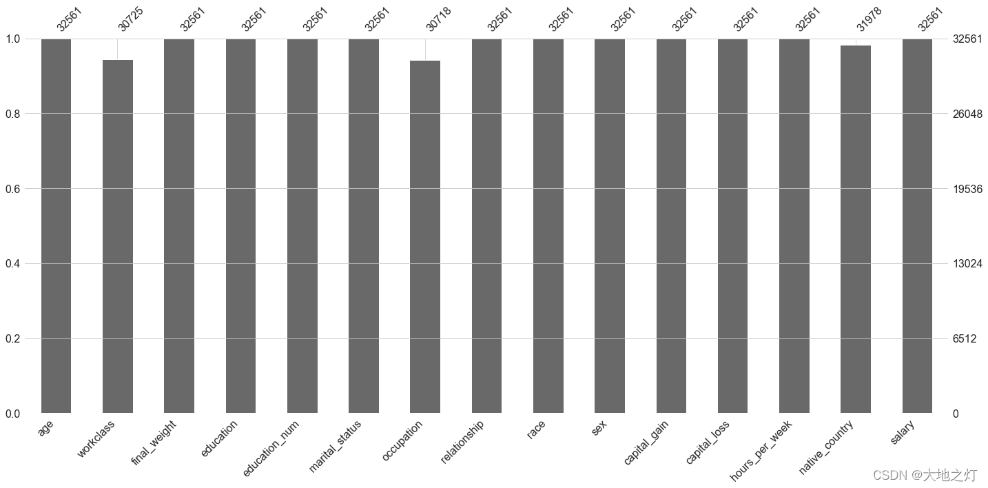
三列有缺失,workclass,occupation,native_country
msno.bar(df)
<AxesSubplot:>
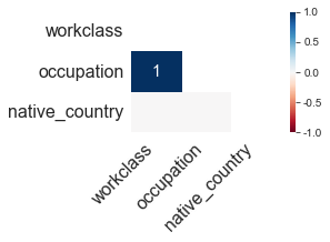
绘制缺失值热力图。利用热力图可以观察多个特征两两的相似度,相似度由皮尔逊相关系数度量。
occupation和workclass为1表明这两个变量在数据集中是同步缺失的。
msno.heatmap(df,figsize=(3,2))
<AxesSubplot:>
分别对训练集和测试集绘制缺失值矩阵图。矩阵图中白线越多,代表缺失值越多。
结果表明workclass和occupation相比于native_country有更多的缺失值
msno.matrix(df,figsize=(6,3))
<AxesSubplot:>
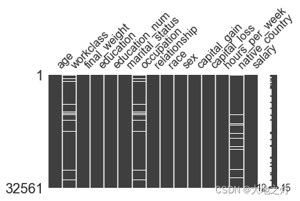
工作类型workclass和职业occupation分别有5.63%和5.66%的缺失,原籍native_country有1.79%缺失
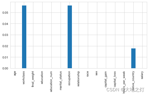
temp = df.apply(lambda x:x.isna().sum()/len(x))
# temp = temp.loc[:,(temp!=0).any()]
temp
age               0.000000
workclass         0.056386
final_weight      0.000000
education         0.000000
education_num     0.000000
marital_status    0.000000
occupation        0.056601
relationship      0.000000
race              0.000000
sex               0.000000
capital_gain      0.000000
capital_loss      0.000000
hours_per_week    0.000000
native_country    0.017905
salary            0.000000
dtype: float64
temp.plot(kind='bar',figsize=(8,4))
<AxesSubplot:>
2.3数据处理 及特征工程
# 判断哪些字段不是数值类型
# X = df.iloc[:,:-1].copy()
# y = df.iloc[:,-1].copy()
# for col_name in X:
#     col_data = X[col_name]
#     if col_data.dtype == 'object':
#         print(col_name,'------->',col_data.unique())

"""
workclass -------> ['State-gov' 'Self-emp-not-inc' 'Private' 'Federal-gov' 'Local-gov' nan
 'Self-emp-inc' 'Without-pay' 'Never-worked']
education -------> ['Bachelors' 'HS-grad' '11th' 'Masters' '9th' 'Some-college' 'Assoc-acdm'
 'Assoc-voc' '7th-8th' 'Doctorate' 'Prof-school' '5th-6th' '10th'
 '1st-4th' 'Preschool' '12th']
marital_status -------> ['Never-married' 'Married-civ-spouse' 'Divorced' 'Married-spouse-absent'
 'Separated' 'Married-AF-spouse' 'Widowed']
occupation -------> ['Adm-clerical' 'Exec-managerial' 'Handlers-cleaners' 'Prof-specialty'
 'Other-service' 'Sales' 'Craft-repair' 'Transport-moving'
 'Farming-fishing' 'Machine-op-inspct' 'Tech-support' nan
 'Protective-serv' 'Armed-Forces' 'Priv-house-serv']
relationship -------> ['Not-in-family' 'Husband' 'Wife' 'Own-child' 'Unmarried' 'Other-relative']
race -------> ['White' 'Black' 'Asian-Pac-Islander' 'Amer-Indian-Eskimo' 'Other']
sex -------> ['Male' 'Female']
native_country -------> ['United-States' 'Cuba' 'Jamaica' 'India' nan 'Mexico' 'South'
 'Puerto-Rico' 'Honduras' 'England' 'Canada' 'Germany' 'Iran'
 'Philippines' 'Italy' 'Poland' 'Columbia' 'Cambodia' 'Thailand' 'Ecuador'
 'Laos' 'Taiwan' 'Haiti' 'Portugal' 'Dominican-Republic' 'El-Salvador'
 'France' 'Guatemala' 'China' 'Japan' 'Yugoslavia' 'Peru'
 'Outlying-US(Guam-USVI-etc)' 'Scotland' 'Trinadad&Tobago' 'Greece'
 'Nicaragua' 'Vietnam' 'Hong' 'Ireland' 'Hungary' 'Holand-Netherlands']
"""
"\nworkclass -------> ['State-gov' 'Self-emp-not-inc' 'Private' 'Federal-gov' 'Local-gov' nan\n 'Self-emp-inc' 'Without-pay' 'Never-worked']\neducation -------> ['Bachelors' 'HS-grad' '11th' 'Masters' '9th' 'Some-college' 'Assoc-acdm'\n 'Assoc-voc' '7th-8th' 'Doctorate' 'Prof-school' '5th-6th' '10th'\n '1st-4th' 'Preschool' '12th']\nmarital_status -------> ['Never-married' 'Married-civ-spouse' 'Divorced' 'Married-spouse-absent'\n 'Separated' 'Married-AF-spouse' 'Widowed']\noccupation -------> ['Adm-clerical' 'Exec-managerial' 'Handlers-cleaners' 'Prof-specialty'\n 'Other-service' 'Sales' 'Craft-repair' 'Transport-moving'\n 'Farming-fishing' 'Machine-op-inspct' 'Tech-support' nan\n 'Protective-serv' 'Armed-Forces' 'Priv-house-serv']\nrelationship -------> ['Not-in-family' 'Husband' 'Wife' 'Own-child' 'Unmarried' 'Other-relative']\nrace -------> ['White' 'Black' 'Asian-Pac-Islander' 'Amer-Indian-Eskimo' 'Other']\nsex -------> ['Male' 'Female']\nnative_country -------> ['United-States' 'Cuba' 'Jamaica' 'India' nan 'Mexico' 'South'\n 'Puerto-Rico' 'Honduras' 'England' 'Canada' 'Germany' 'Iran'\n 'Philippines' 'Italy' 'Poland' 'Columbia' 'Cambodia' 'Thailand' 'Ecuador'\n 'Laos' 'Taiwan' 'Haiti' 'Portugal' 'Dominican-Republic' 'El-Salvador'\n 'France' 'Guatemala' 'China' 'Japan' 'Yugoslavia' 'Peru'\n 'Outlying-US(Guam-USVI-etc)' 'Scotland' 'Trinadad&Tobago' 'Greece'\n 'Nicaragua' 'Vietnam' 'Hong' 'Ireland' 'Hungary' 'Holand-Netherlands']\n"
发现数据存在occupation缺失而workclass为"Never-worked"的情况,反之则不存在。
这是由于无工作者没有职业,此部分可直接将这些occupation填补为一个新的类即可。
df[['occupation','workclass']][(df['occupation'].isna()==True) & (df['workclass'].isna()==False)]
| occupation | workclass | |
|---|---|---|
| 5361 | NaN | Never-worked |
| 10845 | NaN | Never-worked |
| 14772 | NaN | Never-worked |
| 20337 | NaN | Never-worked |
| 23232 | NaN | Never-worked |
| 32304 | NaN | Never-worked |
| 32314 | NaN | Never-worked |
df.loc[df['workclass']=='Never_worked','occupation'] = 'Never_worked'
df['workclass'].value_counts()
Private             22696
Self-emp-not-inc     2541
Local-gov            2093
State-gov            1298
Self-emp-inc         1116
Federal-gov           960
Without-pay            14
Never-worked            7
Name: workclass, dtype: int64
df.head()
| age | workclass | final_weight | education | education_num | marital_status | occupation | relationship | race | sex | capital_gain | capital_loss | hours_per_week | native_country | salary | |
|---|---|---|---|---|---|---|---|---|---|---|---|---|---|---|---|
| 0 | 39 | State-gov | 77516 | Bachelors | 13 | Never-married | Adm-clerical | Not-in-family | White | Male | 2174 | 0 | 40 | United-States | <=50K |
| 1 | 50 | Self-emp-not-inc | 83311 | Bachelors | 13 | Married-civ-spouse | Exec-managerial | Husband | White | Male | 0 | 0 | 13 | United-States | <=50K |
| 2 | 38 | Private | 215646 | HS-grad | 9 | Divorced | Handlers-cleaners | Not-in-family | White | Male | 0 | 0 | 40 | United-States | <=50K |
| 3 | 53 | Private | 234721 | 11th | 7 | Married-civ-spouse | Handlers-cleaners | Husband | Black | Male | 0 | 0 | 40 | United-States | <=50K |
| 4 | 28 | Private | 338409 | Bachelors | 13 | Married-civ-spouse | Prof-specialty | Wife | Black | Female | 0 | 0 | 40 | Cuba | <=50K |
df.sex.value_counts()
Male      21790
Female    10771
Name: sex, dtype: int64
# 处理性别
df['sex'] = 1*(df['sex']=='Male')
df.head()
| age | workclass | final_weight | education | education_num | marital_status | occupation | relationship | race | sex | capital_gain | capital_loss | hours_per_week | native_country | salary | |
|---|---|---|---|---|---|---|---|---|---|---|---|---|---|---|---|
| 0 | 39 | State-gov | 77516 | Bachelors | 13 | Never-married | Adm-clerical | Not-in-family | White | 1 | 2174 | 0 | 40 | United-States | <=50K |
| 1 | 50 | Self-emp-not-inc | 83311 | Bachelors | 13 | Married-civ-spouse | Exec-managerial | Husband | White | 1 | 0 | 0 | 13 | United-States | <=50K |
| 2 | 38 | Private | 215646 | HS-grad | 9 | Divorced | Handlers-cleaners | Not-in-family | White | 1 | 0 | 0 | 40 | United-States | <=50K |
| 3 | 53 | Private | 234721 | 11th | 7 | Married-civ-spouse | Handlers-cleaners | Husband | Black | 1 | 0 | 0 | 40 | United-States | <=50K |
| 4 | 28 | Private | 338409 | Bachelors | 13 | Married-civ-spouse | Prof-specialty | Wife | Black | 0 | 0 | 0 | 40 | Cuba | <=50K |
# 删除education
del df['education']
df.head()
| age | workclass | final_weight | education_num | marital_status | occupation | relationship | race | sex | capital_gain | capital_loss | hours_per_week | native_country | salary | |
|---|---|---|---|---|---|---|---|---|---|---|---|---|---|---|
| 0 | 39 | State-gov | 77516 | 13 | Never-married | Adm-clerical | Not-in-family | White | 1 | 2174 | 0 | 40 | United-States | <=50K |
| 1 | 50 | Self-emp-not-inc | 83311 | 13 | Married-civ-spouse | Exec-managerial | Husband | White | 1 | 0 | 0 | 13 | United-States | <=50K |
| 2 | 38 | Private | 215646 | 9 | Divorced | Handlers-cleaners | Not-in-family | White | 1 | 0 | 0 | 40 | United-States | <=50K |
| 3 | 53 | Private | 234721 | 7 | Married-civ-spouse | Handlers-cleaners | Husband | Black | 1 | 0 | 0 | 40 | United-States | <=50K |
| 4 | 28 | Private | 338409 | 13 | Married-civ-spouse | Prof-specialty | Wife | Black | 0 | 0 | 0 | 40 | Cuba | <=50K |
# 处理salary 标签
df['salary'] = 1*(df['salary']=='>50K')
df.salary.value_counts()
0    24720
1     7841
Name: salary, dtype: int64
df.head(5)
| age | workclass | final_weight | education_num | marital_status | occupation | relationship | race | sex | capital_gain | capital_loss | hours_per_week | native_country | salary | |
|---|---|---|---|---|---|---|---|---|---|---|---|---|---|---|
| 0 | 39 | State-gov | 77516 | 13 | Never-married | Adm-clerical | Not-in-family | White | 1 | 2174 | 0 | 40 | United-States | 0 |
| 1 | 50 | Self-emp-not-inc | 83311 | 13 | Married-civ-spouse | Exec-managerial | Husband | White | 1 | 0 | 0 | 13 | United-States | 0 |
| 2 | 38 | Private | 215646 | 9 | Divorced | Handlers-cleaners | Not-in-family | White | 1 | 0 | 0 | 40 | United-States | 0 |
| 3 | 53 | Private | 234721 | 7 | Married-civ-spouse | Handlers-cleaners | Husband | Black | 1 | 0 | 0 | 40 | United-States | 0 |
| 4 | 28 | Private | 338409 | 13 | Married-civ-spouse | Prof-specialty | Wife | Black | 0 | 0 | 0 | 40 | Cuba | 0 |
temp = df.copy()
# 删除需要独热编码的列,防止列名重复导致编码失败
df.drop(['workclass','marital_status','occupation','relationship','race','native_country'],axis=1,inplace=True)
df.head()
| age | final_weight | education_num | sex | capital_gain | capital_loss | hours_per_week | salary | |
|---|---|---|---|---|---|---|---|---|
| 0 | 39 | 77516 | 13 | 1 | 2174 | 0 | 40 | 0 |
| 1 | 50 | 83311 | 13 | 1 | 0 | 0 | 13 | 0 |
| 2 | 38 | 215646 | 9 | 1 | 0 | 0 | 40 | 0 |
| 3 | 53 | 234721 | 7 | 1 | 0 | 0 | 40 | 0 |
| 4 | 28 | 338409 | 13 | 0 | 0 | 0 | 40 | 0 |
df = df.join(pd.get_dummies(temp.workclass))
df = df.join(pd.get_dummies(temp.marital_status))
df = df.join(pd.get_dummies(temp.occupation))
df = df.join(pd.get_dummies(temp.relationship))
df = df.join(pd.get_dummies(temp.race))
df = df.join(pd.get_dummies(temp.native_country))
df.head()
| age | final_weight | education_num | sex | capital_gain | capital_loss | hours_per_week | salary | Federal-gov | Local-gov | ... | Portugal | Puerto-Rico | Scotland | South | Taiwan | Thailand | Trinadad&Tobago | United-States | Vietnam | Yugoslavia | |
|---|---|---|---|---|---|---|---|---|---|---|---|---|---|---|---|---|---|---|---|---|---|
| 0 | 39 | 77516 | 13 | 1 | 2174 | 0 | 40 | 0 | 0 | 0 | ... | 0 | 0 | 0 | 0 | 0 | 0 | 0 | 1 | 0 | 0 |
| 1 | 50 | 83311 | 13 | 1 | 0 | 0 | 13 | 0 | 0 | 0 | ... | 0 | 0 | 0 | 0 | 0 | 0 | 0 | 1 | 0 | 0 |
| 2 | 38 | 215646 | 9 | 1 | 0 | 0 | 40 | 0 | 0 | 0 | ... | 0 | 0 | 0 | 0 | 0 | 0 | 0 | 1 | 0 | 0 |
| 3 | 53 | 234721 | 7 | 1 | 0 | 0 | 40 | 0 | 0 | 0 | ... | 0 | 0 | 0 | 0 | 0 | 0 | 0 | 1 | 0 | 0 |
| 4 | 28 | 338409 | 13 | 0 | 0 | 0 | 40 | 0 | 0 | 0 | ... | 0 | 0 | 0 | 0 | 0 | 0 | 0 | 0 | 0 | 0 |
5 rows × 89 columns
salary = df.pop('salary')
df['salary'] = salary
df.head()
| age | final_weight | education_num | sex | capital_gain | capital_loss | hours_per_week | Federal-gov | Local-gov | Never-worked | ... | Puerto-Rico | Scotland | South | Taiwan | Thailand | Trinadad&Tobago | United-States | Vietnam | Yugoslavia | salary | |
|---|---|---|---|---|---|---|---|---|---|---|---|---|---|---|---|---|---|---|---|---|---|
| 0 | 39 | 77516 | 13 | 1 | 2174 | 0 | 40 | 0 | 0 | 0 | ... | 0 | 0 | 0 | 0 | 0 | 0 | 1 | 0 | 0 | 0 |
| 1 | 50 | 83311 | 13 | 1 | 0 | 0 | 13 | 0 | 0 | 0 | ... | 0 | 0 | 0 | 0 | 0 | 0 | 1 | 0 | 0 | 0 |
| 2 | 38 | 215646 | 9 | 1 | 0 | 0 | 40 | 0 | 0 | 0 | ... | 0 | 0 | 0 | 0 | 0 | 0 | 1 | 0 | 0 | 0 |
| 3 | 53 | 234721 | 7 | 1 | 0 | 0 | 40 | 0 | 0 | 0 | ... | 0 | 0 | 0 | 0 | 0 | 0 | 1 | 0 | 0 | 0 |
| 4 | 28 | 338409 | 13 | 0 | 0 | 0 | 40 | 0 | 0 | 0 | ... | 0 | 0 | 0 | 0 | 0 | 0 | 0 | 0 | 0 | 0 |
5 rows × 89 columns
2.4 划分数据集
# 判断有没有字段还不是数值类型
X = df.iloc[:,:-1].copy()
y = df.iloc[:,-1].copy()
for col_name in X:
    col_data = X[col_name]
    if col_data.dtype == 'object':
        print(col_name,'------->',col_data.unique())
X.head()
| age | final_weight | education_num | sex | capital_gain | capital_loss | hours_per_week | Federal-gov | Local-gov | Never-worked | ... | Portugal | Puerto-Rico | Scotland | South | Taiwan | Thailand | Trinadad&Tobago | United-States | Vietnam | Yugoslavia | |
|---|---|---|---|---|---|---|---|---|---|---|---|---|---|---|---|---|---|---|---|---|---|
| 0 | 39 | 77516 | 13 | 1 | 2174 | 0 | 40 | 0 | 0 | 0 | ... | 0 | 0 | 0 | 0 | 0 | 0 | 0 | 1 | 0 | 0 |
| 1 | 50 | 83311 | 13 | 1 | 0 | 0 | 13 | 0 | 0 | 0 | ... | 0 | 0 | 0 | 0 | 0 | 0 | 0 | 1 | 0 | 0 |
| 2 | 38 | 215646 | 9 | 1 | 0 | 0 | 40 | 0 | 0 | 0 | ... | 0 | 0 | 0 | 0 | 0 | 0 | 0 | 1 | 0 | 0 |
| 3 | 53 | 234721 | 7 | 1 | 0 | 0 | 40 | 0 | 0 | 0 | ... | 0 | 0 | 0 | 0 | 0 | 0 | 0 | 1 | 0 | 0 |
| 4 | 28 | 338409 | 13 | 0 | 0 | 0 | 40 | 0 | 0 | 0 | ... | 0 | 0 | 0 | 0 | 0 | 0 | 0 | 0 | 0 | 0 |
5 rows × 88 columns
# 无量纲处理 :因为已经使用了哑变量,所以此处不需要无量纲再处理一遍了

from sklearn.preprocessing import StandardScaler
s_X = StandardScaler().fit_transform(X)
s_X = pd.DataFrame(data = s_X,columns = X.columns)
s_X.head()
| age | final_weight | education_num | sex | capital_gain | capital_loss | hours_per_week | Federal-gov | Local-gov | Never-worked | ... | Portugal | Puerto-Rico | Scotland | South | Taiwan | Thailand | Trinadad&Tobago | United-States | Vietnam | Yugoslavia | |
|---|---|---|---|---|---|---|---|---|---|---|---|---|---|---|---|---|---|---|---|---|---|
| 0 | 0.030671 | -1.063611 | 1.134739 | 0.703071 | 0.148453 | -0.21666 | -0.035429 | -0.174295 | -0.262097 | -0.014664 | ... | -0.033729 | -0.059274 | -0.019201 | -0.049628 | -0.039607 | -0.023518 | -0.024163 | 0.340954 | -0.045408 | -0.022173 |
| 1 | 0.837109 | -1.008707 | 1.134739 | 0.703071 | -0.145920 | -0.21666 | -2.222153 | -0.174295 | -0.262097 | -0.014664 | ... | -0.033729 | -0.059274 | -0.019201 | -0.049628 | -0.039607 | -0.023518 | -0.024163 | 0.340954 | -0.045408 | -0.022173 |
| 2 | -0.042642 | 0.245079 | -0.420060 | 0.703071 | -0.145920 | -0.21666 | -0.035429 | -0.174295 | -0.262097 | -0.014664 | ... | -0.033729 | -0.059274 | -0.019201 | -0.049628 | -0.039607 | -0.023518 | -0.024163 | 0.340954 | -0.045408 | -0.022173 |
| 3 | 1.057047 | 0.425801 | -1.197459 | 0.703071 | -0.145920 | -0.21666 | -0.035429 | -0.174295 | -0.262097 | -0.014664 | ... | -0.033729 | -0.059274 | -0.019201 | -0.049628 | -0.039607 | -0.023518 | -0.024163 | 0.340954 | -0.045408 | -0.022173 |
| 4 | -0.775768 | 1.408176 | 1.134739 | -1.422331 | -0.145920 | -0.21666 | -0.035429 | -0.174295 | -0.262097 | -0.014664 | ... | -0.033729 | -0.059274 | -0.019201 | -0.049628 | -0.039607 | -0.023518 | -0.024163 | -2.932948 | -0.045408 | -0.022173 |
5 rows × 88 columns
from sklearn.model_selection import train_test_split
X_train,X_test,y_train,y_test = train_test_split(s_X,y)
2.5 训练
1.随机森林
from sklearn.model_selection import GridSearchCV
from sklearn.ensemble import RandomForestClassifier
# 随机森林调参,跑了几个小时才跑完
# RF = RandomForestClassifier()
# param_grid = {'max_features':['auto','sqrt','log2'],
#               'max_depth':np.arange(1,15),
#               'min_samples_leaf':np.arange(1,20),
#               'min_samples_split':[0.1,0.3,0.5],
#               'criterion':['gini','entropy']
#              }
# GS = GridSearchCV(RF,param_grid=param_grid,cv=5,scoring='roc_auc').fit(x_train,y_train)
# print(GS.best_params_)
# print(GS.best_score_)
# print(GS.best_estimator_)

"""
{'criterion': 'gini', 'max_depth': 12, 'max_features': 'auto', 'min_samples_leaf': 1, 'min_samples_split': 0.1}
0.9044572707834764
RandomForestClassifier(max_depth=12, min_samples_split=0.1)
"""
"\n{'criterion': 'gini', 'max_depth': 12, 'max_features': 'auto', 'min_samples_leaf': 1, 'min_samples_split': 0.1}\n0.9044572707834764\nRandomForestClassifier(max_depth=12, min_samples_split=0.1)\n"
RF = RandomForestClassifier(criterion='gini', max_depth = 12, max_features='auto', min_samples_leaf = 3, min_samples_split = 0.1).fit(X_train,y_train)
RF.score(X_test,y_test)
0.844490848790075
from sklearn.metrics import classification_report
print(classification_report(y_test,RF.predict(X_test)))
              precision    recall  f1-score   support

           0       0.85      0.96      0.90      6194
           1       0.79      0.47      0.59      1947

    accuracy                           0.84      8141
   macro avg       0.82      0.72      0.75      8141
weighted avg       0.84      0.84      0.83      8141
2 SVM 支持向量机
from sklearn import svm
svc_bal = svm.SVC(class_weight='balanced')  #自动调整不平衡样本
svc_bal.fit(X_train,y_train)
SVC(class_weight='balanced')
svc_bal.score(X_test,y_test)
0.8030954428202923
print(classification_report(y_test,svc_bal.predict(X_test)))
              precision    recall  f1-score   support

           0       0.94      0.80      0.86      6194
           1       0.56      0.83      0.67      1947

    accuracy                           0.80      8141
   macro avg       0.75      0.81      0.76      8141
weighted avg       0.85      0.80      0.81      8141
3 逻辑回归
from sklearn.linear_model import LogisticRegression
lr = LogisticRegression()
lr.fit(X_train,y_train)
LogisticRegression()
print(classification_report(y_test,lr.predict(X_test)))
              precision    recall  f1-score   support

           0       0.88      0.93      0.91      6194
           1       0.74      0.61      0.67      1947

    accuracy                           0.86      8141
   macro avg       0.81      0.77      0.79      8141
weighted avg       0.85      0.86      0.85      8141
lr.score(X_test,y_test)
0.8560373418498956
from sklearn.model_selection import cross_val_score
from sklearn.model_selection import GridSearchCV
# 网格搜索过程,比较耗时,为方便调试先注释起来
"""
param_grid = {
    'C':[0.01, 0.1,1, 10,20],
    'penalty':['l1','l2'],
    'max_iter':[50, 100, 200, 300,500,1000]
}
gscv = GridSearchCV(estimator=LogisticRegression(),param_grid=param_grid,cv=10)
gscv.fit(ss_X,y)
gscv.best_params_
"""
# 最优参数
# {'C': 0.01, 'max_iter': 50, 'penalty': 'l2'}
"\nparam_grid = {\n 'C':[0.01, 0.1,1, 10,20],\n 'penalty':['l1','l2'],\n 'max_iter':[50, 100, 200, 300,500,1000]\n}\ngscv = GridSearchCV(estimator=LogisticRegression(),param_grid=param_grid,cv=10)\ngscv.fit(ss_X,y)\ngscv.best_params_\n"
# 使用cross_val_score 来进行预测评分
# estimator 算法对象
# X, y = None 特征向量集合 标签集合
# cv Kfold的几折 3 5 10
lr = LogisticRegression(C=0.01,max_iter=50,penalty='l2')
result = cross_val_score(lr,X,y,cv=10)
result
array([0.79643844, 0.80006143, 0.79361179, 0.79637592, 0.79453317,
       0.80773956, 0.79084767, 0.80128993, 0.79668305, 0.79821867])
result.mean()
0.7975799619643648
4 Adaboost
from sklearn.ensemble import AdaBoostClassifier
from sklearn.tree import DecisionTreeClassifier
ada = AdaBoostClassifier(
    base_estimator = DecisionTreeClassifier(max_depth=2),
    n_estimators=50,
    learning_rate=1.0
).fit(X_train,y_train)
print(classification_report(y_test,ada.predict(X_test)))
              precision    recall  f1-score   support

           0       0.90      0.94      0.92      6194
           1       0.76      0.66      0.71      1947

    accuracy                           0.87      8141
   macro avg       0.83      0.80      0.81      8141
weighted avg       0.87      0.87      0.87      8141
ada.score(X_test,y_test)
0.8700405355607419
5 GDBT
from sklearn.ensemble import GradientBoostingClassifier
gbdt = GradientBoostingClassifier().fit(X_train,y_train)
print(classification_report(y_test,gbdt.predict(X_test)))
              precision    recall  f1-score   support

           0       0.88      0.95      0.92      6194
           1       0.80      0.60      0.69      1947

    accuracy                           0.87      8141
   macro avg       0.84      0.78      0.80      8141
weighted avg       0.86      0.87      0.86      8141
6 XGB
from xgboost import XGBClassifier
from xgboost import XGBRegressor
sk_xgb_c = XGBClassifier().fit(X_train,y_train)
print(classification_report(y_test,sk_xgb_c.predict(X_test)))
              precision    recall  f1-score   support

           0       0.90      0.94      0.92      6194
           1       0.77      0.65      0.71      1947

    accuracy                           0.87      8141
   macro avg       0.83      0.80      0.81      8141
weighted avg       0.87      0.87      0.87      8141


 2568
2568


 被折叠的 条评论
为什么被折叠?
被折叠的 条评论
为什么被折叠?
 到【灌水乐园】发言


