多目标蚁群算法路径规划（四）------多目标约束过程常规流程框架

热力学负一定理

于 2022-01-03 19:06:21 发布

阅读量8.9k

点赞数 18

分类专栏：路径规划汇总文集文章标签：算法 matlab 路径规划

本文链接：https://blog.csdn.net/qq_33980829/article/details/122287240

版权

路径规划汇总文集专栏收录该内容

11 篇文章

订阅专栏

多目标蚁群算法路径规划（四）

文章目录

多目标蚁群算法路径规划（四）
零、系列前言（一定要看）
一、内容说明
- 1.1 本章内容说明
- 1.2 本章主要分享内容简介(摘要)
二. 多目标计算预先准备
三、完整多目标求解结果过程展示
四。相关的求解代码

零、系列前言（一定要看）

本系列为总结本人近2年多关于启发式算法解决路径规划的相关内容。主要从以下几个主题内容进行系列写作1.常见的数据获取方式与处理过程、，2、算法的基础流程，3.常见算法改进，4.多目标排序、5.基于应用场景的改进、6.其他相关问题、7、批量运行测试数据本系列全程免费提供相关代码。
本系列代码来源主要参考网上相关博客与文献、根据不同实际需求重构的代码。
本文所有提供的代码与文字说明仅供参考，不作为商业目的。
对内容有疑问或是错误部分可以留言或私信。
有偿定制特定功能, qq:1602480875。价格范围60—500。（建议优先看完系列内容，尝试系列中的代码，这些都是免费且能解决大部分问题。），具体代码后续会以完整形式上传百度云。
更新时间：2022年1月2日
全文共33000字建议收藏

一、内容说明

1.1 本章内容说明

多目标计算的原因
多目标求解的预先的准备
多目标计算的流程
计算结果展示与部分代码分享。
一个完整流程结果的展示
下期预告

1.2 本章主要分享内容简介(摘要)

一个真实环境的决策过程中通常包含不止一个目标需要满足最优条件，而且这些目标之间还存在相互矛盾与制约。为了权衡（trades-off）不同目标的最优条件，决策过程退而求其次计算出目标最优的包络曲线（帕累托最优解）。我们希望获得的规划结果在多个角度都是约束条件中最优的且我们可以根据实际的需求选择帕累托曲线上的点。
首先本文第一部分介绍进行多目标规划时候需要考虑的问题，确认问题是否有必要考虑多目标设计。以及常用的多目标选择以及需要注意的事项，针对常用的多目标算法进行分享说明与常用算法框架
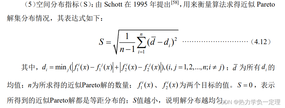
第二部分本文是对多目标算法的比对与结果评价的常用方法进行总结。相比单目标只需比较的最终目标的大小，多目标的比较方法相对复杂通常用的方法包括：1.权衡曲线分析，2.取非支配真实总体，3.错误率，4.空间分布指标（非支配总体数量（NOVG）、非支配真实总体数量（OTNVG）、非支配真实总体率（OTNVGR）、失误率（ER）、空间分布指标（S））等。最后总结不同多目标算法设计思路的特点与局限性。
第三部分展示一个完整的多目标规划流程结果：1. 数据设计，2. 数据划分，3.多目标路径规划，4.计算帕累托非支配前沿解，5.对计算后的线路根据车辆数目约束求调度结果，6.算法结果评价

二. 多目标计算预先准备

2.1 多目标规划时候需要考虑的问题

1. 明确目标函数之间的权衡关系

我们在设计多目标评价函数时首先需要考虑的是选择的的目标之间是否有线性相关性，这个部分是决定后续求解过程中排序结果的分布。通常我们在文献中经常看到最短路径和碳排放或是最小成本同时作为目标函数，如果只是简单将两者组合就容易导致出现典型的没有考虑目标的线性相关关系缺少判断。这也是经常导致结果不理想，数据结果难以解释。
例如：
$最短路径=\sum 车辆行驶距离$
$碳排放 = 车辆行驶总距离 \times 二氧化碳排放$
$成本 = 距离 * 油价 + 车辆数目 * 固定消耗$
上述两者数学上都与路径长度线性相关，在导致求解的最优解只会有一个方向，不存在权衡的过程。只需要将两者合并转化成本作为一个与行驶距离相关的单目标函数函数.这种情况下没必要考虑成多目标函数进行设计。

2. 目标函数的设计

那么如何设计一个好的多目标函数呢？我们还是以上述两个目标函数为例考虑，对目标函数进行修改。
首先重新思考车辆碳排放的过程是否除了路径相关还与其他什么联系，比如：1.考虑车辆运输载重对碳排放的权重是否同等于或是大于行驶路径的长度。2.车辆的频繁启动与停留是否也是重要需要考虑的因素。当我们考虑在两个条件后就会使碳排放成本不完全与行驶路径距离相关，并非路径越短就会使碳排放越低。两者可以出现相互制约的结果，有时路径长而碳排放则表现为较低的水平（如图）。同时单次规划上路径点的个数也是制约的目标求解的限制因素。

在这里插入图片描述

$最短路径=\sum 车辆线路$
$碳排放 = f u n c t i o n （车辆载重，行驶距离） \times 二氧化碳排放 + f u n c t i o n 2 （路径经过点数目）$

3. 常用的目标函数选择

本文整理了一些常用的多目标函数，但在具体实际应用过程中需要根据问题背景进行考虑。1）满意度与成本，2）路径长度与碳排放 3）成本与调度等（待补充，也可留言补充）。
在这里插入图片描述

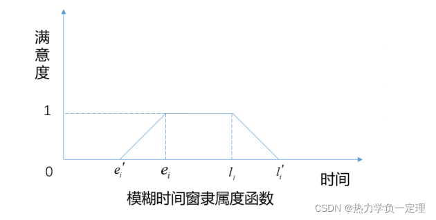
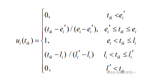
满意度计算模型：
在这里插入图片描述

2.2. 常用求解多目标算法

1. 算法综述

目前常用的多目标求解算法包括线性求解器直接计算，通过启发式算法求解例如：NSGA-Ⅱ，NSGA-Ⅲ，MDVRPTW-Ⅱ等。其核心部分都是通过启发算法获得初始解，通过非支配排序过程对启发是求解的结果进行排序分层。根据每一层排序结果进行下一轮的重新迭代，以此多次迭代得到多目标排序结果。然后将排序结果绘制帕累托非支配解，根据实际需求求解出最优的前沿解。
请添加图片描述

在这里插入图片描述

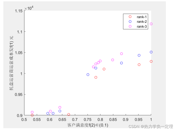
2. 不同多目标算法的比对

采用非支配总体数量（NOVG）、非支配真实总体数量（OTNVG）、非支配真实总体率（OTNVGR）、失误
率（ER）、空间分布指标（S）五个评价指标，评价算法性能优劣。

非支配总体数量（NOVG）：表示非支配解集中解的个数。非支配解集中的
解的数量越多，表示此算法对特定场景下的问题求解时，可以得到更多的解，解的多
样性越好，非支配解集越优。
非支配真实总体数量（OTNVG）：指非支配解集中的可行解在此特定问题下标准解集的数量。此评价指标与非支配解集中较差的解集无关，表示运行算法得到的非支配解集中最优解的个数。
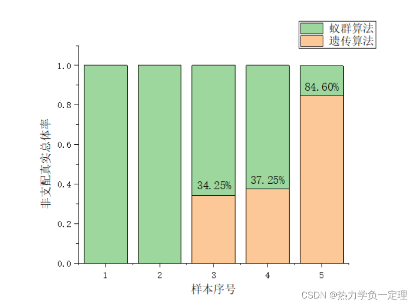
非支配真实总体率（OTNVGR）：表示非支配真实总体数量占此特定问题标准解集中的百分比。此指标有效防止了对于不同问题的标准解集的数量不同，从而使非支配真实总体数量指标失效的问题。例如：运行蚁群算法和遗传算法得出的帕累托前沿解，经过再次非支配排序，共同构成了此问题的标准解集（包含 10 个解），其中蚁群算法的帕累托前沿解集中有 6 个解与标准解集重复，那么蚁群算法运算结果的非支配真实总体率为百分之 60%。
失误率（ER）：该指标由 Van Veldhuizen 提出，指的是非支配解集中可行解不在最优解集中解的个数，占标准解集的百分比。

在这里插入图片描述

三、完整多目标求解结果过程展示

过程中涉及的相关实现过程可以参照本系列前面已经发表的博客进行对照。本文的结果全部来源博主个人完成的实例。

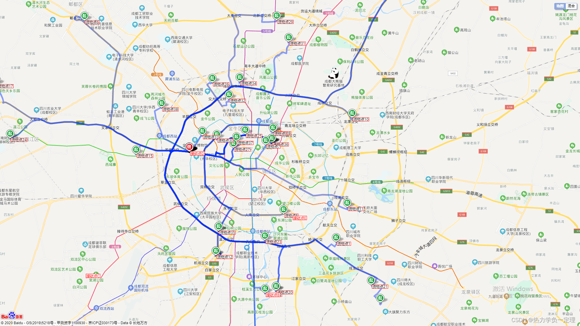
3.1 数据获取

基于百度地图API获取实际路径距离与经纬度坐标

3.2 数据预处理

将获取的数据转化处理，区域划分

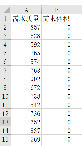
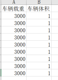
3.2 约束条件整理

设置约束条件与需求

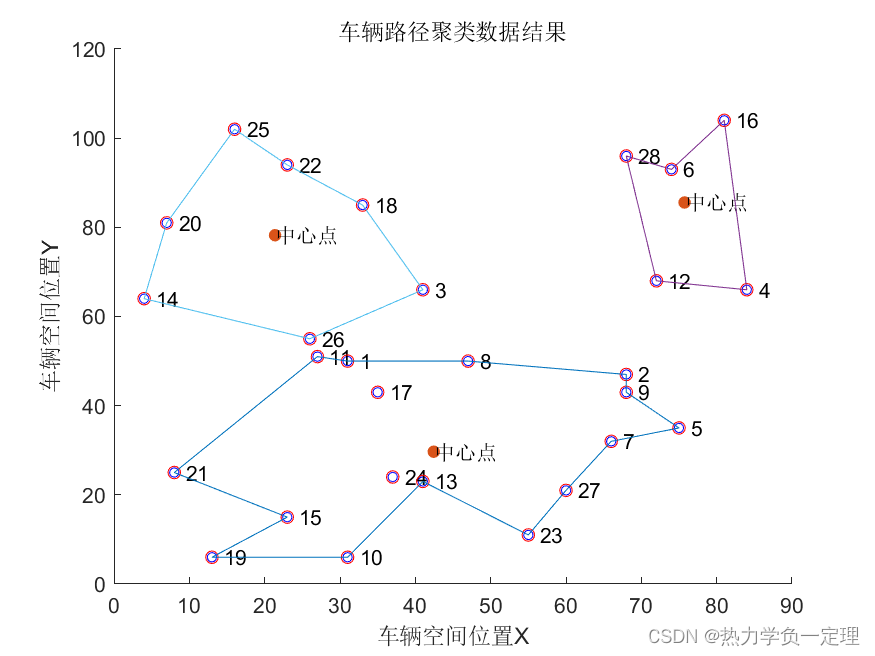
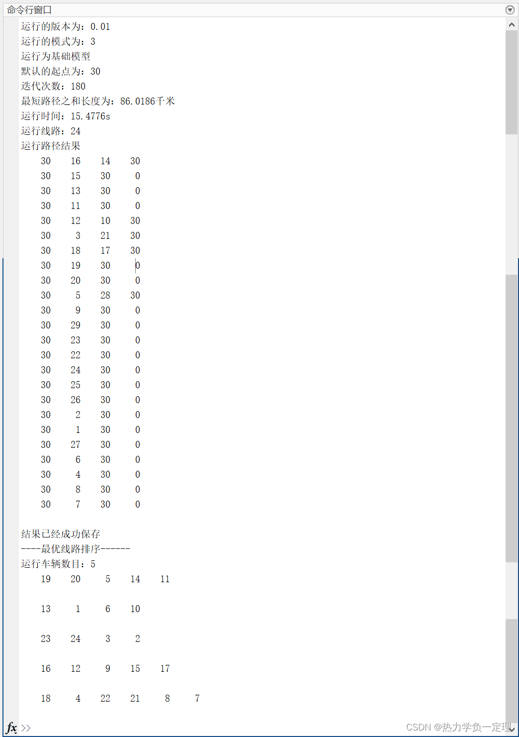
3.3 初步运行求解

区域内求解结果划分求解规划路径
比较求解过程的迭代稳定性与收敛性优化参数设置

在这里插入图片描述

3.4 启发式参数设计优化

- 在这里插入图片描述

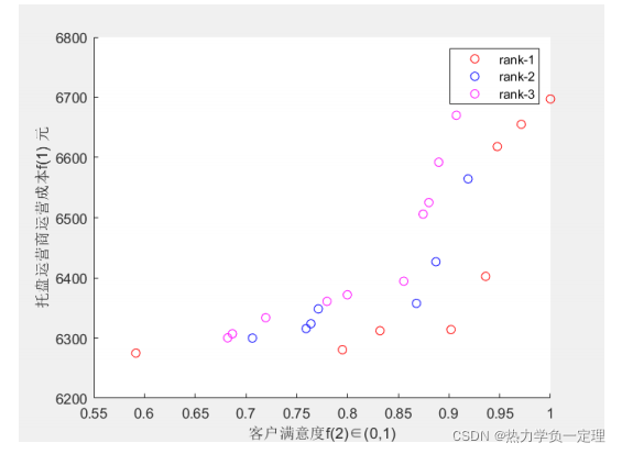
3.5 多目标求解的怕累托排序

将多目标规划结果进行帕累托排序，获取前沿解

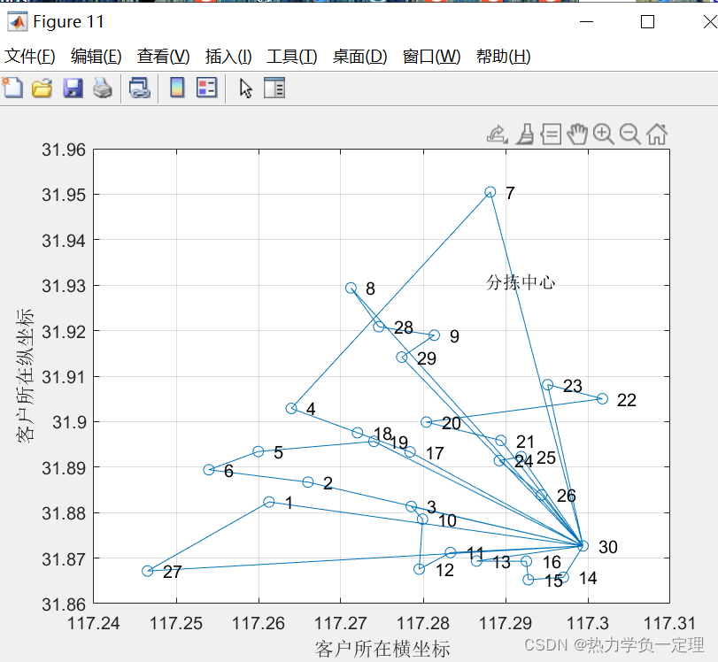
3.6 路径求解结果的调度优化

根据帕累托前沿解获取路径规划结果，绘制最优车辆线路调度

3.7 规划结果的分析讨论

获取最优线路与最优发车顺序结果

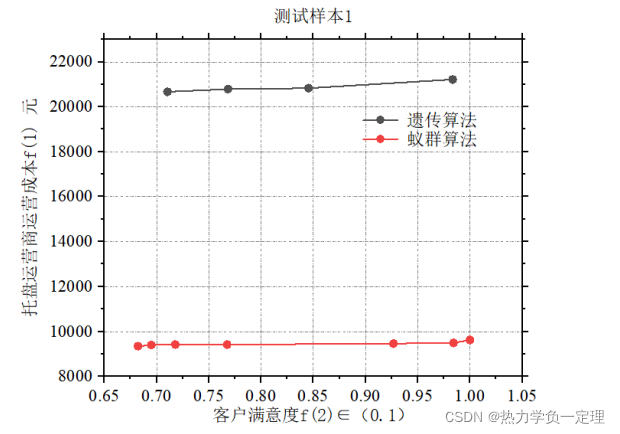
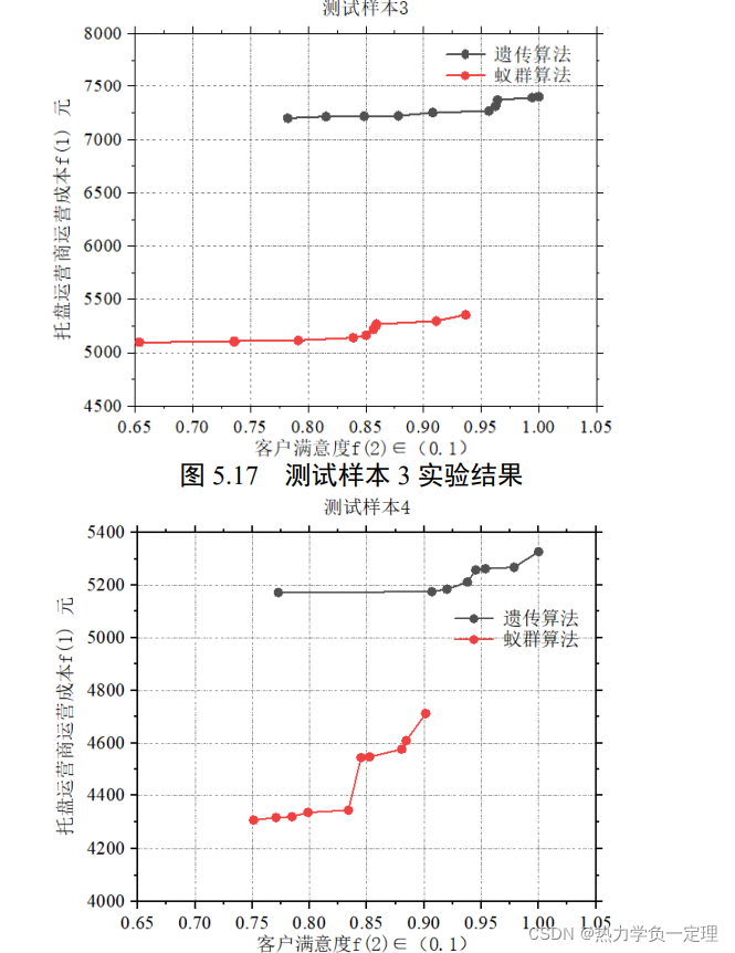
3.8 优化改进算法与多算法比对

在这里插入图片描述

3.9 根据问题背景多角度改进优化

请添加图片描述

3.10 经典数据集的运算与总结

在这里插入图片描述

四。相关的求解代码

4.1 蚁群多目标路径求解

clc
clear
close all
% 主程序
for i=2:9
      a='H:\软件安装包\项目文件\交通规划项目结果图\蚁群算法规划\工作簿1.xlsx';%文件地址
    [x2,D,Cap,C,d_u,t1,v_2,cost_2]=fist_1(5,a);
    D=D(1:i,1:i);
    Demand=zeros(size(D,1),2);
    Alpha=1;Beta=5; %
    Rho=0.75; % 
    iter_max=100; %迭代次数
    Q=10;   %
    m=size(D,1);  %起始放置数目
    qidian=1;  % qidian起点坐标
     [R_best,L_best,L_ave,Shortest_Route,Shortest_Length,j_1_j]=ANT_VRP_1(D,Demand,Cap,iter_max,m,Alpha,Beta,Rho,Q,qidian,d_u,t1,v_2,cost_2,x2);
    Shortest_Route_1=Shortest_Route;    %提取最优路线
    cc=find(Shortest_Route_1==qidian);
    xx_1=[];
    if length(cc)==2
        for i=1:1
            cs_1=length(Shortest_Route_1(cc(i):cc(i+1)));
            xx_1(i,1:cs_1)=Shortest_Route_1(cc(i):cc(i+1)); %路线
        end
    else
        for i=1:length(cc)/2+2
            cs_1=length(Shortest_Route_1(cc(i):cc(i+1)));
            xx_1(i,1:cs_1)=Shortest_Route_1(cc(i):cc(i+1)); %路线
        end
    end
    Shortest_Length;                      %提取最短路径长度

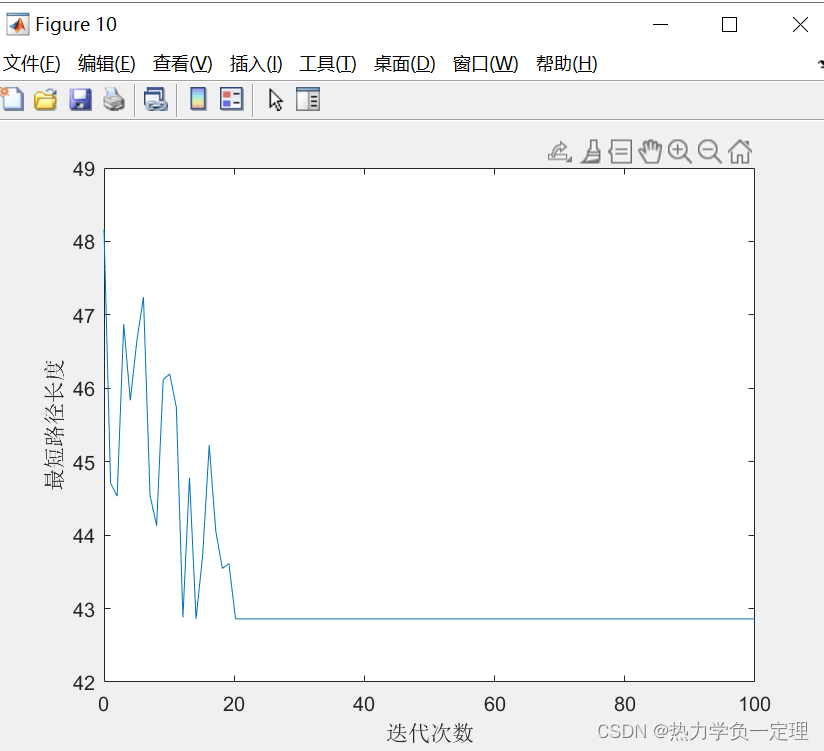
    %% ==============作图==============
%     figure(1)   %作迭代收敛曲线图
%     x=linspace(0,iter_max,iter_max);
%     y=L_best(:,1); 
%     plot(x,y);
%     xlabel('迭代次数'); ylabel('最短路径长度');

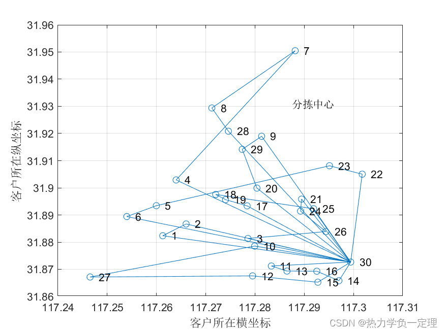
    figure(2)   %作最短路径图
    plot(C(Shortest_Route,1),C(Shortest_Route,2),'o-');
    grid on
    for i =1:size(C,1)
        if i==qidian
            text(C(i,1),C(i,2),' 起始港口 ');
        else
            text(C(i,1),C(i,2),['   ' num2str(i)]);
        end
    end
    xlabel('客户所在横坐标'); ylabel('客户所在纵坐标');
   hold on
 best_all(i)=1/Shortest_Length;
 for i=1:length(Shortest_Route)-1
    tim_1(i)=t1(Shortest_Route(i),Shortest_Route(i+1));
end
    time_all=sum(tim_1);
end
hold off
disp("最后收益为：")
disp(strcat(num2str(max(best_all)),'元'))
disp("最后需要经历的港口数目：")
disp(num2str(find(best_all==max(best_all))))
disp("运行的时间：")
disp(strcat(num2str(time_all),'天'))
disp("运行的顺序：")
disp(Shortest_Route)
 
 figure 
 for i =1:size(C,1)
        if i==qidian
            text(C(i,1),C(i,2),' 起始港口 ');
        else
            text(C(i,1),C(i,2),['   ' num2str(i)]);
        end
end
    xlabel('客户所在横坐标'); ylabel('客户所在纵坐标');

function ACO_VRPTW(all_name_sys)
%% 多目标批量计算
%% 版本0.1
%% 时间
% clear
% clc
% close all
tic

%% 输入数据解析
filepath=all_name_sys.filepath;
foler=all_name_sys.foler;
stad_pint=all_name_sys.stad_pint;
output_data_name=all_name_sys.output_data_name;
num_file_data=all_name_sys.num_file;
%% 用importdata这个函数来读取文件
c101=xlsread(foler);
%% 调试时使用
% p= mfilename('fullpath');
% [filepath,name,ext] = fileparts(p);
% c101=importdata('c104_1.txt');
% % 如果第一行不是起点，运行下面代码
% stad_pint=[ 0  86         51          0          0       1236          0   ];
% c101=[stad_pint;c101];
if c101(1,1)~=0
    disp('已设置起点')
    c101=[stad_pint;c101];
end
cap=600000;                                                     %车辆最大装载量
v_cap=2;   %车辆速度（单位时间）
%% 锟斤拷取锟斤拷锟斤拷锟斤拷息
E=c101(1,5);                                                   %配送中心时间窗开始时间
L=c101(1,6);                                                    %配送中心时间窗结束时间
pint_list_name=c101(:,1);%名称坐标
vertexs=c101(:,2:3);                                            %所有点的坐标x和y
customer=vertexs(2:end,:);                                      %顾客坐标
cusnum=size(customer,1);                                       %顾客数
v_num=25;                                                       %车辆最多使用数目
demands=c101(2:end,4);                                          %需求量
a=c101(2:end,5);                                                %顾客时间窗开始时间[a[i],b[i]]
b=c101(2:end,6);                                                %顾客时间窗结束时间[a[i],b[i]]
time_x=[a,b];%时间
width=b-a;                                                       %顾客的时间窗宽度
s=c101(2:end,7);                                                 %客户点的服务时间
choose_way=input('计算的距离类型————1 坐标位置 2 经纬度===');
if choose_way==1
    h=pdist(vertexs);
    dist=squareform(h);                                            %距离矩阵 坐标相减
    % dist(1,3)=555;
else
%     mi=vertexs;
%     cc=zeros(size(mi,1));
%     for j=1:size(mi,1)
%         for i=j:size(mi,1)
%             cc(j,i)=abs(6371004*acos((sin(deg2rad(mi(j,2)))*sin(deg2rad(mi(i,2)))+cos(deg2rad(mi(j,2)))*cos(deg2rad(mi(i,2)))*cos(deg2rad(mi(i,1)-mi(j,1))))));
%             if i==j || cc(j,i)==0
% %                 cc(j,i)=eps;
%  cc(j,i)=0;
%             end
%             cc(i,j)=cc(j,i);
%         end
%     end
%     un_1_1=cc;
% 
%     a=a*40;
%     b=b*40;
    time_x=[a,b];%时间
    width=b-a;
 D = Haversin(vertexs);
    dist=D;        %距离矩阵
end
%% 锟斤拷始锟斤拷锟斤拷锟斤拷
w_PPm_b=1;%锟斤拷始锟斤拷锟斤拷锟轿?1
m=100;                                                             %蚂蚁数量
alpha=1;                                                        %信息素重要程度因子
beta=3;                                                        %启发函数重要程度因子
gama=2;                                                          %等待时间重要程度因子
delta=3;                                                       %时间窗跨度重要程度因子
r0=0.5;                                                        %r0为用来控制转移规则的参数
rho=0.85;                                                         %信息素挥发因子
Q=100;                                                           %更新信息素浓度的常数
Eta=1./dist;                                                    %启发函数
Tau=ones(cusnum+1,cusnum+1);                                   %信息素矩阵
Table=zeros(m,cusnum);                                          %路径记录表
iter=1;                                                         %迭代次数初值
iter_max=2;                                                   %最大迭代次数
Route_best=zeros(iter_max,cusnum);                            %各代最佳路径
Cost_best=zeros(iter_max,1);                                      %各代最佳路径的成本
%% 迭代寻找最佳路径
while iter<=iter_max
    %% 先构建出所有蚂蚁的路径
    %逐个蚂蚁选择
    for i=1:m
        %逐个顾客选择
        for j=1:cusnum
            r=rand;                                             %r为在[0,1]上的随机变量
            np=next_point(i,Table,Tau,Eta,alpha,beta,gama,delta,r,r0,a,b,width,s,L,dist,cap,demands);
            Table(i,j)=np;
        end
    end
    % cw节约算法 初始化 以路径和载重为约束
    if iter==1
        A = [vertexs';0 demands'];
        %         D = Haversin(a);
        D=dist;
        lorry=cap;
%         Table = zeros(m,cusnum);
        Table(1,:) = CW(A,D,lorry);
%         clear A D lorry
    end
    %% 计算各个蚂蚁的成本=1000*车辆使用数目+车辆行驶总距离
    cost=zeros(m,1);
    NV=zeros(m,1);
    TD=zeros(m,1);
 %成本计算方法1
    for i=1:m
        [VC,NV,TD,Q_U,w_pp]=decode(Table(i,:),cap,demands,a,b,L,s,dist);
        [cost(i,1),NV(i,1),TD(i,1),ff(i,1),c_11(i,1),w_PPm(i,1)]=costFun(VC,dist,Q_U,w_pp);           
    end
%成本计算方法2
%     for iix=1:m
%         [fit(iix,:),err(iix,:)]=test_case(Table(iix,:),dist,demands',time_x,lorry);
%         cost(iix,1)=fit(iix,1);
%         w_PPm(iix,1)=fit(iix,2);
%     end
    %% 计算最小成本及平均成本
    % 成本计算1
    if iter == 1
        [min_Cost,min_index]=min(cost);
        c_bb=c_11(min_index);
        f_bb=ff(min_index);
        Cost_best(iter)=min_Cost;
        w_PPm_m(iter)=mean(w_PPm);
        Route_best(iter,:)=Table(min_index,:);
    else
        [min_Cost,min_index]=min(cost);
        w_PPm_m(iter)=mean(w_PPm);
        Cost_best(iter)=min(Cost_best(iter - 1),min_Cost);
        c_bb=c_11(min_index);
        f_bb=ff(min_index);
        w_PPm_b=w_PPm(min_index);
        if Cost_best(iter)==min_Cost
            Route_best(iter,:)=Table(min_index,:);
            c_bb=c_11(min_index);
            f_bb=ff(min_index);
            w_PPm_b=w_PPm(min_index);
        else
            Route_best(iter,:)=Route_best((iter-1),:);
            c_bb=c_11(min_index);
            f_bb=ff(min_index);
            w_PPm_b=w_PPm(min_index);
        end
   
        %% 非支持排序主体
%         all_data_try_1=[Table,1-w_PPm,cost]; %多目标指标
        %成本二
         all_data_try_1=[Table,w_PPm,cost]; %多目标指标
        [m_lings,n_lings]=sort(all_data_try_1(:,end), 'descend','MissingPlacement','last' );
        all_data_try=all_data_try_1(n_lings,:);
        save(strcat(filepath,'/data/all_data_try',num2str(iter),'.mat'),'all_data_try')
        if iter<3
            all_data_try_ST=all_data_try;
            save(strcat(filepath,'/data/aLL_data_try_aLL',num2str(num_file_data),'.mat'),'all_data_try_ST')
        else
            load(strcat(filepath,'/data/aLL_data_try_aLL',num2str(num_file_data),'.mat'))
            all_data_try_ST=[all_data_try_ST;all_data_try];
            save(strcat(filepath,'/data/aLL_data_try_aLL',num2str(num_file_data),'.mat'),'all_data_try_ST')
        end
        set_num.star_Scale_factor=0.5;%初始迭代选择数目
        set_num.every_Scale_factor=0.9;%每次运算比例
        set_num.gen = 99; %迭代次数
        set_num.M = 2; %目标函数数量
        set_num.mu = 0.5;  %选取的数目的比例
        set_num.mum = 2; %是否随机 1 随机 2不随机
        set_num.num_file_data=num_file_data; % 运行的文件编号
        file_name_1=strcat('data/all_data_try',num2str(iter),'.mat');% 当前运行结果
        file_name_2=strcat(filepath,'/data/aLL_data_try_aLL',num2str(num_file_data),'.mat'); %当前运行结果
%         p_NSGA_2=nsga_2(file_name_1,file_name_2,set_num);
        %         save(strcat('Table_',num2str(iter),'.mat'),'Table')
        %         save(strcat('w_PPm',num2str(iter),'.mat'),'w_PPm')
        %         save(strcat('cost',num2str(iter),'.mat'),'cost')
    end
    %% 更新信息素
    bestR=Route_best(iter,:);
    [bestVC,bestNV,bestTD]=decode(bestR,cap,demands,a,b,L,s,dist);
    Tau=updateTau(Tau,bestR,rho,Q,cap,demands,a,b,L,s,dist);
    %% 最短时间
    t_1=bestTD/v_cap;% 路径时间
    s_1=sum(s); % 总服务时间
    T_BEAST=t_1+s_1;
    %% 打印当前最优解
    disp(['第',num2str(iter),'代最优解:'])
    disp(['车辆使用数目',num2str(bestNV),'车辆行驶总距离：',num2str(bestTD),'最低碳排放量',num2str(c_bb),'满意度为',num2str(w_PPm_b),'最短时间',num2str(T_BEAST)]);
    
    fprintf('\n')
    
    %% 迭代次数加1，清空路径记录表
    iter=iter+1;
    Table=zeros(m,cusnum);
end
%% 结果显示
a_time=now;
bestRoute=Route_best(end,:);
[bestVC,NV,TD]=decode(bestRoute,cap,demands,a,b,L,s,dist);
draw_Best(bestVC,vertexs,pint_list_name);
clear LD
for i=1:size(bestVC,1)
    [~,LD(i)]=begin_cap_thng(bestVC{i},demands,cap); %每次出发携带的最低货物量
end
save(strcat(output_data_name,'bestVC.mat'),'bestVC','vertexs','pint_list_name','LD')
fig_name=strcat(output_data_name,'路径变化图',date,'_',num2str(a_time),'.fig');
savefig(gcf,fig_name)
%% 绘图
figure(2)
plot(1:iter_max,Cost_best,'b')
xlabel('迭代次数')
ylabel('成本')
title('各代最小成本变化趋势图')
fig_name=strcat(output_data_name,'各代最小成本变化趋势图',date,'_',num2str(a_time),'.fig');
savefig(gcf,fig_name)
% %% 判断最优解是否满足时间窗约束和载重量约束，0表示违反约束，1表示满足全部约束
% flag=Judge(bestVC,cap,demands,a,b,L,s,dist);
%% 检查最优解中是否存在元素丢失的情况，丢失元素，如果没有则为空
% DEL=Judge_Del(bestVC);
figure(3)
plot(1:iter_max,w_PPm_m,'b')
xlabel('迭代次数')
ylabel('满意度')
title('各代满意度平均变化趋势图')
fig_name=strcat(output_data_name,'各代满意度平均变化趋势图',date,'_',num2str(a_time),'.fig');
savefig(gcf,fig_name)
figure(4)
plot(1:m,w_PPm,'b')
xlabel('蚂蚁')
ylabel('满意度')
title('最后一代满意度平均变化趋势图')
fig_name=strcat(output_data_name,'最后一代满意度平均变化趋势图',date,'_',num2str(a_time),'.fig');
savefig(gcf,fig_name)
toc

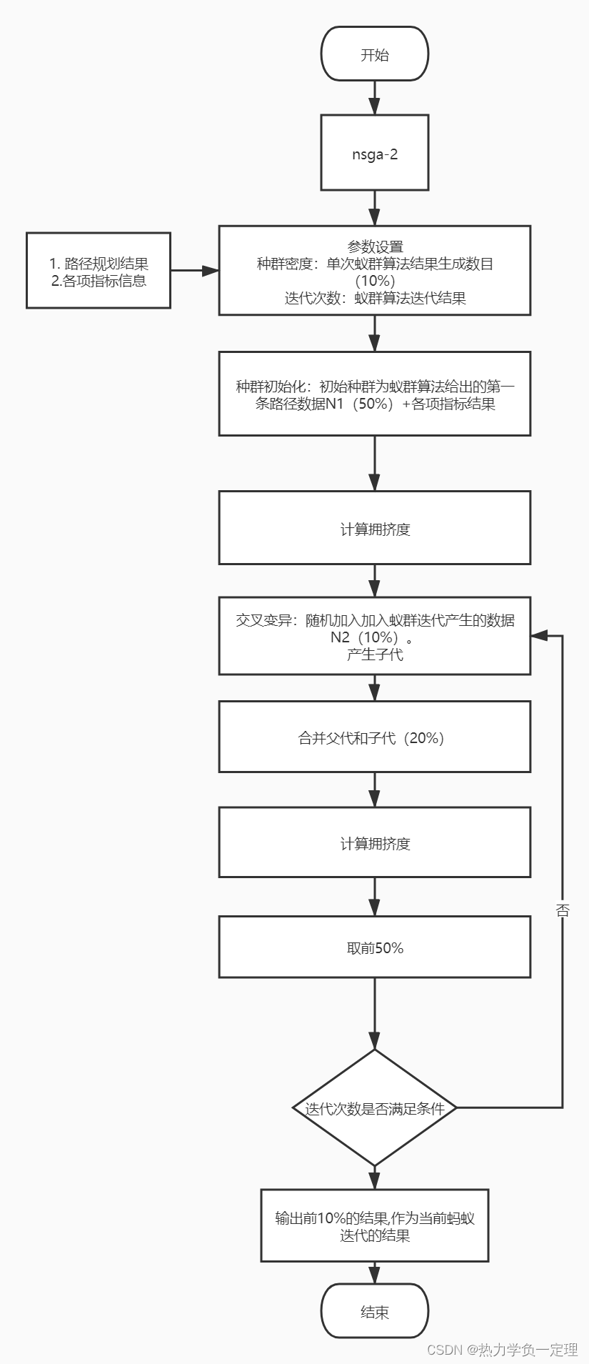
4.2 蚁群多目标路径求解非支配排序主函数

function chromosome=nsga_2(file_name_1,file_name_2,set_num)

%% function nsga_2(pop,gen)
% is a multi-objective optimization function where the input arguments are
% pop - Population size
% gen - Total number of generations
%
% This functions is based on evolutionary algorithm for finding the optimal
% solution for multiple objective i.e. pareto front for the objectives.
% Initially enter only the population size and the stoping criteria or
% the total number of generations after which the algorithm will
% automatically stopped.
%
% You will be asked to enter the number of objective functions, the number
% of decision variables and the range space for the decision variables.
% Also you will have to define your own objective funciton by editing the
% evaluate_objective() function. A sample objective function is described
% in evaluate_objective.m. Kindly make sure that the objective function
% which you define match the number of objectives that you have entered as
% well as the number of decision variables that you have entered. The
% decision variable space is continuous for this function, but the
% objective space may or may not be continuous.
%
% Original algorithm NSGA-II was developed by researchers in Kanpur Genetic
% Algorithm Labarotary and kindly visit their website for more information
% http://www.iitk.ac.in/kangal/


%  Copyright (c) 2009, Aravind Seshadri
%  All rights reserved.
%
%  Redistribution and use in source and binary forms, with or without
%  modification, are permitted provided that the following conditions are
%  met:
%
%     * Redistributions of source code must retain the above copyright
%       notice, this list of conditions and the following disclaimer.
%     * Redistributions in binary form must reproduce the above copyright
%       notice, this list of conditions and the following disclaimer in
%       the documentation and/or other materials provided with the distribution
%
%  THIS SOFTWARE IS PROVIDED BY THE COPYRIGHT HOLDERS AND CONTRIBUTORS "AS IS"
%  AND ANY EXPRESS OR IMPLIED WARRANTIES, INCLUDING, BUT NOT LIMITED TO, THE
%  IMPLIED WARRANTIES OF MERCHANTABILITY AND FITNESS FOR A PARTICULAR PURPOSE
%  ARE DISCLAIMED. IN NO EVENT SHALL THE COPYRIGHT OWNER OR CONTRIBUTORS BE
%  LIABLE FOR ANY DIRECT, INDIRECT, INCIDENTAL, SPECIAL, EXEMPLARY, OR
%  CONSEQUENTIAL DAMAGES (INCLUDING, BUT NOT LIMITED TO, PROCUREMENT OF
%  SUBSTITUTE GOODS OR SERVICES; LOSS OF USE, DATA, OR PROFITS; OR BUSINESS
%  INTERRUPTION) HOWEVER CAUSED AND ON ANY THEORY OF LIABILITY, WHETHER IN
%  CONTRACT, STRICT LIABILITY, OR TORT (INCLUDING NEGLIGENCE OR OTHERWISE)
%  ARISING IN ANY WAY OUT OF THE USE OF THIS SOFTWARE, EVEN IF ADVISED OF THE
%  POSSIBILITY OF SUCH DAMAGE.

%% Simple error checking
% Number of Arguments
% Check for the number of arguments. The two input arguments are necessary
% to run this function.
% if nargin < 2
%     error('NSGA-II: Please enter the population size and number of generations as input arguments.');
% end
% % Both the input arguments need to of integer data type
% if isnumeric(pop) == 0 || isnumeric(gen) == 0
%     error('Both input arguments pop and gen should be integer datatype');
% end
% % Minimum population size has to be 20 individuals
% if pop < 20
%     error('Minimum population for running this function is 20');
% end
% if gen < 5
%     error('Minimum number of generations is 5');
% end
% % Make sure pop and gen are integers
% pop = round(pop);
% gen = round(gen);
%% Objective Function
% The objective function description contains information about the
% objective function. M is the dimension of the objective space, V is the
% dimension of decision variable space, min_range and max_range are the
% range for the variables in the decision variable space. User has to
% define the objective functions using the decision variables. Make sure to
% edit the function 'evaluate_objective' to suit your needs.
%% 鏁版嵁杈撳叆
% [M, V, min_range, max_range] = objective_description_function();
%% 浠ｇ爜娴嬭瘯
%姹傜殑鏄渶灏忕殑鍊?
% load('铓佺兢绠楁硶/璺緞瑙勫垝/data/all_data_try2.mat');
load(file_name_1)
data_1=all_data_try;
star_Scale_factor=set_num.star_Scale_factor;
every_Scale_factor=set_num.every_Scale_factor;
gen=set_num.gen;
num_file_data=set_num.num_file_data;
M=set_num.M;
% star_Scale_factor=0.5;%鍒濆杩唬閫夋嫨鏁扮洰
% every_Scale_factor=0.9;%姣忔杩愮畻姣斾緥
size_data=size(data_1,1); %杈撳叆鐨勭粨鏋滄暟鐩?
pop = ceil(every_Scale_factor*size(data_1,1)); %绉嶇兢鏁伴噺
% gen = 99; %杩唬娆℃暟
% M = 2; %鐩爣鍑芥暟鏁伴噺
V = size(data_1,2)-M; %缁村害锛堝喅绛栧彉閲忕殑涓暟锛?
% min_range = zeros(1, V); %涓嬬晫 鐢熸垚1*30鐨勪釜浣撳悜閲? 鍏ㄤ负0
% max_range = ones(1,V); %涓婄晫 鐢熸垚1*30鐨勪釜浣撳悜閲? 鍏ㄤ负1
%% Initialize the population
% Population is initialized with random values which are within the
% specified range. Each chromosome consists of the decision variables. Also
% the value of the objective functions, rank and crowding distance
% information is also added to the chromosome vector but only the elements
% of the vector which has the decision variables are operated upon to
% perform the genetic operations like corssover and mutation.
chromosome = initialize_variables(data_1,star_Scale_factor); %鍒濆鍖?


%% Sort the initialized population
% Sort the population using non-domination-sort. This returns two columns
% for each individual which are the rank and the crowding distance
% corresponding to their position in the front they belong. At this stage
% the rank and the crowding distance for each chromosome is added to the
% chromosome vector for easy of computation.
chromosome = non_domination_sort_mod(chromosome, M, V); %闈炴敮閰嶈В

%% Start the evolution process
% The following are performed in each generation
% * Select the parents which are fit for reproduction
% * Perfrom crossover and Mutation operator on the selected parents
% * Perform Selection from the parents and the offsprings
% * Replace the unfit individuals with the fit individuals to maintain a
%   constant population size.

for i = 1 : gen
    % Select the parents
    % Parents are selected for reproduction to generate offspring. The
    % original NSGA-II uses a binary tournament selection based on the
    % crowded-comparision operator. The arguments are
    % pool - size of the mating pool. It is common to have this to be half the
    %        population size.
    % tour - Tournament size. Original NSGA-II uses a binary tournament
    %        selection, but to see the effect of tournament size this is kept
    %        arbitary, to be choosen by the user.
    pool = round(pop/2);
    tour = 2;
    % Selection process
    % A binary tournament selection is employed in NSGA-II. In a binary
    % tournament selection process two individuals are selected at random
    % and their fitness is compared. The individual with better fitness is
    % selcted as a parent. Tournament selection is carried out until the
    % pool size is filled. Basically a pool size is the number of parents
    % to be selected. The input arguments to the function
    % tournament_selection are chromosome, pool, tour. The function uses
    % only the information from last two elements in the chromosome vector.
    % The last element has the crowding distance information while the
    % penultimate element has the rank information. Selection is based on
    % rank and if individuals with same rank are encountered, crowding
    % distance is compared. A lower rank and higher crowding distance is
    % the selection criteria.
    parent_chromosome = tournament_selection(chromosome, every_Scale_factor, star_Scale_factor,data_1,size_data,gen,i,M); %浜ゅ弶鍙樺紓閫夋嫨
    
    % Perfrom crossover and Mutation operator
    % The original NSGA-II algorithm uses Simulated Binary Crossover (SBX) and
    % Polynomial  mutation. Crossover probability pc = 0.9 and mutation
    % probability is pm = 1/n, where n is the number of decision variables.
    % Both real-coded GA and binary-coded GA are implemented in the original
    % algorithm, while in this program only the real-coded GA is considered.
    % The distribution indeices for crossover and mutation operators as mu = 20
    % and mum = 20 respectively.
    %浜ゅ弶鍙樺紓
    
    if exist(file_name_2)~=0
        file_name=file_name_2; %姹犲寲瑙ｇ殑鑼冨洿
        mu=set_num.mu;
        mum=set_num.mum;
        %             mu = 0.5;  %閫塋ine 170 %             mu = 0.5;  %閫夊彇鐨勬暟鐩殑姣斾緥
        
        %             mum = 2; %鏄惁闅忔満 1 闅忔満 2涓嶉殢鏈?
        %          disp('浜ゅ弶')
        offspring_chromosome = genetic_operator(parent_chromosome, M, V, mu, mum,file_name);%浜ゅ弶鎵╁緛
    else
        %          disp('涓嶄氦鍙?')
        offspring_chromosome=[parent_chromosome;parent_chromosome];
    end
    
    % Intermediate population
    % Intermediate population is the combined population of parents and
    % offsprings of the current generation. The population size is two
    % times the initial population.
    
    [main_pop,temp] = size(chromosome);
    [offspring_pop,temp] = size(offspring_chromosome);
    % temp is a dummy variable.
    clear temp
    % intermediate_chromosome is a concatenation of current population and
    % the offspring population.
    intermediate_chromosome(1:main_pop,:) = chromosome;
    intermediate_chromosome(main_pop + 1 : main_pop + offspring_pop,1 : M+V) = ...
        offspring_chromosome;
    % Non-domination-sort of intermediate population
    % The intermediate population is sorted again based on non-domination sort
    % before the replacement operator is performed on the intermediate
    % population.
    intermediate_chromosome=unique(intermediate_chromosome,'row');
    intermediate_chromosome = ...
        non_domination_sort_mod(intermediate_chromosome, M, V);
    % Perform Selection
    % Once the intermediate population is sorted only the best solution is
    % selected based on it rank and crowding distance. Each front is filled in
    % ascending order until the addition of population size is reached. The
    % last front is included in the population based on the individuals with
    % least crowding distance
    chromosome = replace_chromosome(intermediate_chromosome, M, V, pop);
    %     chromosome(:,v)=abs(chromosome(:,1:end-M));
    if ~mod(i,100)
        clc
        fprintf('%d generations completed\n',i);
    end
end

%% Result
% Save the result in ASCII text format.
% save solution.txt chromosome -ASCII
% num_file_data
save('solution.mat','chromosome')
if exist(strcat('top_chromosome_1',num2str(num_file_data),'.mat'))~=0
    load(strcat('top_chromosome_1',num2str(num_file_data),'.mat'))
    top_chromosome=top_chromosome_1;
    top_chromosome_1=chromosome(1:ceil(0.1*size(chromosome,1)),:);
    top_chromosome_1=[top_chromosome;top_chromosome_1];
    save(strcat('top_chromosome_1',num2str(num_file_data),'.mat'),'top_chromosome_1')
else
    top_chromosome_1=chromosome(1:ceil(1*size(chromosome,1)),:);
    save(strcat('top_chromosome_1',num2str(num_file_data),'.mat'),'top_chromosome_1')
end


%% Visualize
% The following is used to visualize the result if objective space
% dimension is visualizable.
% if M == 2
%     plot(chromosome(:,V + 1),chromosome(:,V + 2),'*');
% elseif M ==3
%     plot3(chromosome(:,V + 1),chromosome(:,V + 2),chromosome(:,V + 3),'*');
% end

4.3 非支配排序

function f = non_domination_sort_mod(x, M, V)

%% function f = non_domination_sort_mod(x, M, V)
% This function sort the current popultion based on non-domination. All the
% individuals in the first front are given a rank of 1, the second front
% individuals are assigned rank 2 and so on. After assigning the rank the
% crowding in each front is calculated.

%  Copyright (c) 2009, Aravind Seshadri
%  All rights reserved.
%
%  Redistribution and use in source and binary forms, with or without 
%  modification, are permitted provided that the following conditions are 
%  met:
%
%     * Redistributions of source code must retain the above copyright 
%       notice, this list of conditions and the following disclaimer.
%     * Redistributions in binary form must reproduce the above copyright 
%       notice, this list of conditions and the following disclaimer in 
%       the documentation and/or other materials provided with the distribution
%      
%  THIS SOFTWARE IS PROVIDED BY THE COPYRIGHT HOLDERS AND CONTRIBUTORS "AS IS" 
%  AND ANY EXPRESS OR IMPLIED WARRANTIES, INCLUDING, BUT NOT LIMITED TO, THE 
%  IMPLIED WARRANTIES OF MERCHANTABILITY AND FITNESS FOR A PARTICULAR PURPOSE 
%  ARE DISCLAIMED. IN NO EVENT SHALL THE COPYRIGHT OWNER OR CONTRIBUTORS BE 
%  LIABLE FOR ANY DIRECT, INDIRECT, INCIDENTAL, SPECIAL, EXEMPLARY, OR 
%  CONSEQUENTIAL DAMAGES (INCLUDING, BUT NOT LIMITED TO, PROCUREMENT OF 
%  SUBSTITUTE GOODS OR SERVICES; LOSS OF USE, DATA, OR PROFITS; OR BUSINESS 
%  INTERRUPTION) HOWEVER CAUSED AND ON ANY THEORY OF LIABILITY, WHETHER IN 
%  CONTRACT, STRICT LIABILITY, OR TORT (INCLUDING NEGLIGENCE OR OTHERWISE) 
%  ARISING IN ANY WAY OUT OF THE USE OF THIS SOFTWARE, EVEN IF ADVISED OF THE 
%  POSSIBILITY OF SUCH DAMAGE.

[N, m] = size(x);
clear m

% Initialize the front number to 1.
front = 1;

% There is nothing to this assignment, used only to manipulate easily in
% MATLAB.
F(front).f = [];
individual = [];

%% Non-Dominated sort. 
% The initialized population is sorted based on non-domination. The fast
% sort algorithm [1] is described as below for each

% � for each individual p in main population P do the following
%   � Initialize Sp = []. This set would contain all the individuals that is
%     being dominated by p.
%   � Initialize np = 0. This would be the number of individuals that domi-
%     nate p.
%   � for each individual q in P
%       * if p dominated q then
%           � add q to the set Sp i.e. Sp = Sp ? {q}
%       * else if q dominates p then
%           � increment the domination counter for p i.e. np = np + 1
%   � if np = 0 i.e. no individuals dominate p then p belongs to the first
%     front; Set rank of individual p to one i.e prank = 1. Update the first
%     front set by adding p to front one i.e F1 = F1 ? {p}
% � This is carried out for all the individuals in main population P.
% � Initialize the front counter to one. i = 1
% � following is carried out while the ith front is nonempty i.e. Fi != []
%   � Q = []. The set for storing the individuals for (i + 1)th front.
%   � for each individual p in front Fi
%       * for each individual q in Sp (Sp is the set of individuals
%         dominated by p)
%           � nq = nq?1, decrement the domination count for individual q.
%           � if nq = 0 then none of the individuals in the subsequent
%             fronts would dominate q. Hence set qrank = i + 1. Update
%             the set Q with individual q i.e. Q = Q ? q.
%   � Increment the front counter by one.
%   � Now the set Q is the next front and hence Fi = Q.
%
% This algorithm is better than the original NSGA ([2]) since it utilize
% the informatoion about the set that an individual dominate (Sp) and
% number of individuals that dominate the individual (np).

%
for i = 1 : N
    % Number of individuals that dominate this individual
    individual(i).n = 0;
    % Individuals which this individual dominate
    individual(i).p = [];
    for j = 1 : N
        dom_less = 0;
        dom_equal = 0;
        dom_more = 0;
        for k = 1 : M
            if (x(i,V + k) < x(j,V + k))
                dom_less = dom_less + 1;
            elseif (x(i,V + k) == x(j,V + k))
                dom_equal = dom_equal + 1;
            else
                dom_more = dom_more + 1;
            end
        end
        if dom_less == 0 && dom_equal ~= M
            individual(i).n = individual(i).n + 1;
        elseif dom_more == 0 && dom_equal ~= M
            individual(i).p = [individual(i).p j];
        end
    end   
    if individual(i).n == 0
        x(i,M + V + 1) = 1;
        F(front).f = [F(front).f i];
    end
end
% Find the subsequent fronts
while ~isempty(F(front).f)
   Q = [];
   for i = 1 : length(F(front).f)
       if ~isempty(individual(F(front).f(i)).p)
        	for j = 1 : length(individual(F(front).f(i)).p)
            	individual(individual(F(front).f(i)).p(j)).n = ...
                	individual(individual(F(front).f(i)).p(j)).n - 1;
        	   	if individual(individual(F(front).f(i)).p(j)).n == 0
               		x(individual(F(front).f(i)).p(j),M + V + 1) = ...
                        front + 1;
                    Q = [Q individual(F(front).f(i)).p(j)];
                end
            end
       end
   end
   front =  front + 1;
   F(front).f = Q;
end

[temp,index_of_fronts] = sort(x(:,M + V + 1));
for i = 1 : length(index_of_fronts)
    sorted_based_on_front(i,:) = x(index_of_fronts(i),:);
end
current_index = 0;

%% Crowding distance
%The crowing distance is calculated as below
% � For each front Fi, n is the number of individuals.
%   � initialize the distance to be zero for all the individuals i.e. Fi(dj ) = 0,
%     where j corresponds to the jth individual in front Fi.
%   � for each objective function m
%       * Sort the individuals in front Fi based on objective m i.e. I =
%         sort(Fi,m).
%       * Assign infinite distance to boundary values for each individual
%         in Fi i.e. I(d1) = ? and I(dn) = ?
%       * for k = 2 to (n ? 1)
%           � I(dk) = I(dk) + (I(k + 1).m ? I(k ? 1).m)/fmax(m) - fmin(m)
%           � I(k).m is the value of the mth objective function of the kth
%             individual in I

% Find the crowding distance for each individual in each front
for front = 1 : (length(F) - 1)
%    objective = [];
    distance = 0;
    y = [];
    previous_index = current_index + 1;
    for i = 1 : length(F(front).f)
        y(i,:) = sorted_based_on_front(current_index + i,:);
    end
    current_index = current_index + i;
    % Sort each individual based on the objective
    sorted_based_on_objective = [];
    for i = 1 : M
        [sorted_based_on_objective, index_of_objectives] = ...
            sort(y(:,V + i));
        sorted_based_on_objective = [];
        for j = 1 : length(index_of_objectives)
            sorted_based_on_objective(j,:) = y(index_of_objectives(j),:);
        end
        f_max = ...
            sorted_based_on_objective(length(index_of_objectives), V + i);
        f_min = sorted_based_on_objective(1, V + i);
        y(index_of_objectives(length(index_of_objectives)),M + V + 1 + i)= Inf;
        y(index_of_objectives(1),M + V + 1 + i) = Inf;
         for j = 2 : length(index_of_objectives) - 1
            next_obj  = sorted_based_on_objective(j + 1,V + i);
            previous_obj  = sorted_based_on_objective(j - 1,V + i);
            if (f_max - f_min == 0)
                y(index_of_objectives(j),M + V + 1 + i) = Inf;
            else
                y(index_of_objectives(j),M + V + 1 + i) = ...
                     (next_obj - previous_obj)/(f_max - f_min);
            end
         end
    end
    distance = [];
    distance(:,1) = zeros(length(F(front).f),1);
    for i = 1 : M
        distance(:,1) = distance(:,1) + y(:,M + V + 1 + i);
    end
    y(:,M + V + 2) = distance;
    y = y(:,1 : M + V + 2);
    z(previous_index:current_index,:) = y;
end
f = z();

%% References
% [1] *Kalyanmoy Deb, Amrit Pratap, Sameer Agarwal, and T. Meyarivan*, |A Fast
% Elitist Multiobjective Genetic Algorithm: NSGA-II|, IEEE Transactions on 
% Evolutionary Computation 6 (2002), no. 2, 182 ~ 197.
%
% [2] *N. Srinivas and Kalyanmoy Deb*, |Multiobjective Optimization Using 
% Nondominated Sorting in Genetic Algorithms|, Evolutionary Computation 2 
% (1994), no. 3, 221 ~ 248.