


前言
上一篇博客中提到了部分边缘检测算子,不过还有几个更先进的边缘检测算子没有写上。这也是为后续开展图像轮廓等实验做准备。
Marr-Hildreth(LOG算子)
其实这个算子就是高斯平滑与拉普拉斯的结合。其原理:由于灰度变化与图像尺度无关,因此可以使用不同尺度的微分算子进行边缘检测,大尺度微分算子可以检测模糊的边缘,小尺度微分算子可以检测清晰的细节。
选择拉普拉斯算子的两个基本思想:(1)算子的高斯部分会模糊图像,导致灰度结构(包括噪声)的尺度减小到远小于 σ \sigma σ。(2)拉普拉斯的二阶导数性质,尽管一阶导数可用于检测灰度突变,但他们是方向性算子。
另外,拉普拉斯有着各向同性(旋转不变)的重要有点,这不仅符合人的视觉系统特性,而且对任何该方向的灰度变化的响应是相等的,从而避免了使用多个核去计算图像中任意点处的最强响应。
二维高斯函数: G ( x , y ) = e − x 2 + y 2 2 σ 2 G(x,y)=e^{-\frac{x^2+y^2}{2\sigma^2}} G(x,y)=e−2σ2x2+y2
用 ∇ 2 \nabla^2 ∇2表示拉普拉斯,G表示标准差为 δ \delta δ的二维高斯核函数。
G ( x , y ) = ∂ 2 G ( x , y ) ∂ x 2 + ∂ 2 G ( x , y ) ∂ y 2 = ∂ ∂ x ( − x ∂ 2 e − x 2 + y 2 2 ∂ 2 ) + ∂ ∂ y ( − y ∂ 2 e − x 2 + y 2 2 ∂ 2 ) = ( x 2 ∂ 4 − 1 ∂ 2 ) e − x 2 + y 2 2 ∂ 2 + ( y 2 ∂ 4 − 1 ∂ 2 ) e − x 2 + y 2 2 ∂ 2 G(x,y)=\frac{{\partial}^2G(x,y)}{\partial x^2}+\frac{{\partial}^2G(x,y)}{\partial y^2}=\frac{\partial}{\partial x}(\frac{-x}{{\partial}^2}e^{-\frac{x^2+y^2}{2{\partial}^2}})+\frac{\partial}{\partial y}(\frac{-y}{{\partial}^2}e^{-\frac{x^2+y^2}{2{\partial}^2}})=(\frac{x^2}{{\partial}^4}-\frac{1}{{\partial}^2})e^{-\frac{x^2+y^2}{2{\partial}^2}}+(\frac{y^2}{{\partial}^4}-\frac{1}{{\partial}^2})e^{-\frac{x^2+y^2}{2{\partial}^2}} G(x,y)=∂x2∂2G(x,y)+∂y2∂2G(x,y)=∂x∂(∂2−xe−2∂2x2+y2)+∂y∂(∂2−ye−2∂2x2+y2)=(∂4x2−∂21)e−2∂2x2+y2+(∂4y2−∂21)e−2∂2x2+y2
∇ 2 G ( x , y ) = ( x 2 + y 2 − 2 ∂ 2 ∂ 4 ) e − x 2 + y 2 2 ∂ 2 {\nabla}^2G(x,y)=(\frac{x^2+y^2-2{\partial}^2}{{\partial}^4})e^{-\frac{x^2+y^2}{2{\partial}^2}} ∇2G(x,y)=(∂4x2+y2−2∂2)e−2∂2x2+y2
这个就是高斯拉普拉斯(LOG)函数。
算法具体情况如下:首先让LOG核与一幅输入图像卷积。 g ( x , y ) = [ ∇ 2 G ( x , y ) ] ∗ f ( x , y ) g(x,y)=[{\nabla}^2G(x,y)]\ast f(x,y) g(x,y)=[∇2G(x,y)]∗f(x,y)
然后寻找 g ( x , y ) g(x,y) g(x,y)的过零点来确定 f ( x , y ) f(x,y) f(x,y)中边缘的位置。因为拉普拉斯变换核卷积都是线性于是暖,因此可以将上式写为: g ( x , y ) = [ ∇ 2 G ( x , y ) ∗ f ( x , y ) ] g(x,y)=[{\nabla}^2G(x,y)\ast f(x,y)] g(x,y)=[∇2G(x,y)∗f(x,y)]
此处星号 ∗ \ast ∗表示卷积运算。
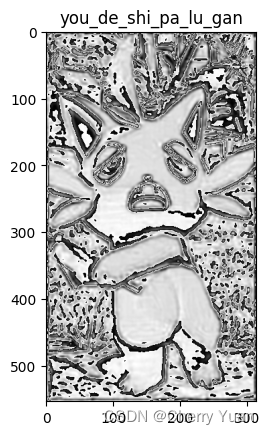
因此,LOG算子的具体实现:可以先对图像做高斯平滑,再做拉普拉斯变换;也可以利用卷积运算的结合律,先计算高斯拉普拉斯卷积核,再与图像卷积,以提高计算速度。
#先做高斯平滑,再做拉普拉斯变换
import numpy as np
import matplotlib.pyplot as plt
from PIL import Image

img = Image.open("go_work.jpg")
plt.title("ni_bu_gan")
plt.imshow(img,cmap="brg")
plt.show()

img_gray = img.convert("L")
plt.title("dao_dan_mao")
plt.imshow(img_gray,cmap="gray")
plt.show()

image = np.array(img_gray)

#高斯平滑
def GaussianBlur(sigma):
    ksize = 2 * (3 * sigma) + 1
    filter = np.ones((ksize,ksize)) / (ksize ** 2)
    for i in range(ksize):
        for j in range(ksize):
            filter[i,j] = np.exp((((i - 3 * sigma) ** 2) + (j - 3 * sigma) ** 2) * (-1)/(sigma ** 2 * 2))
    return filter

#卷积之前的填充
def padding_image(image,h_f,w_f):
    h_img,w_img = image.shape
    h_new,w_new = h_img + h_f - 1,w_img + w_f - 1
    image_padding = np.zeros((h_new,w_new))
    for i in range(h_img):
        for j in range(w_img):
            image_padding[i + int((h_f-1)/2),j + int((w_f-1)/2)] = image[i,j]
    return image_padding

#无论是相关运算,还是卷积运算,经过滤波器核之后的图像输出结果

#空间卷积运算,注意:这里的d一定是偶数
def convolution_operation(image,filter):
    h_img,w_img = image.shape
    h_f,w_f = filter.shape
    filter_convolution = np.flip(filter)#卷积运算所需二维核是对相关运算二维核的翻转。
    image_out = np.zeros((h_img,w_img))
    image_padding = padding_image(image,h_f,w_f)

    for i in range(h_img):
        for j in range(w_img):
            image_out[i,j] = np.sum(np.multiply(filter_convolution[:,:],image_padding[i:i+h_f,j:j+w_f]))
    return image_out

#高斯平滑后的图像
def img_Gauss(image,sigma):
    return convolution_operation(image,GaussianBlur(sigma))

#拉普拉斯变换
def img_Laplacian(img_arr):
    h,w = img_arr.shape

    img_laplacian_ori = np.zeros((h,w))
    laplacian_ori = np.zeros((h,w))

    filter_laplacian_ori = np.matrix([[1,1,1],[1,-8,1],[1,1,1]])
    for i in range(1,h-1):
        for j in range(1,w-1):
            laplacian_ori[i,j] = abs(np.sum(np.multiply(img_arr[i-1:i+2,j-1:j+2],filter_laplacian_ori)))

    return laplacian_ori

#绘图
def draw_convolution(sigma):
    image_convolution = img_Laplacian(img_Gauss(image,sigma))
    image_out = np.uint8(image_convolution)

    plt.title("you_de_shi_pa_lu_gan")
    plt.imshow(image_out,cmap="gray")
    plt.show()

if __name__ == "__main__":
    sigma = 2
    draw_convolution(sigma)


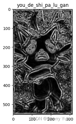
接下来需要徒手写拉普拉斯高斯平滑了,这里面需要注意的是,此处使用的拉普拉斯高斯滤波器的大小不再是预先给定好的,如拉普拉斯滤波器那般。此处滤波器的大小是由 σ \sigma σ值决定的,因为LOG算子规定了滤波器中心点以外的其他点与中心点的距离最大不超过 2 σ \sqrt{2}\sigma 2σ。
既然如此,那么我们接下来就顶风行事,直接让滤波器的大小为 2 ∗ 3 ∗ σ + 1 2*3*\sigma+1 2∗3∗σ+1。这样一来, σ \sigma σ一定得是正整数了,当然这也是我举个例子,作为特殊情况,大家自己做的时候可以自己定大小,但一定要在 2 ∗ 3 ∗ σ + 1 2*3*\sigma+1 2∗3∗σ+1的范围内。我这里的设置的滤波器中心点的坐标就是 ( 3 σ , 3 σ ) (3\sigma,3\sigma) (3σ,3σ)。
注意,这里用半径为 3 σ 3\sigma 3σ,是考虑到高斯标准差确定滤波核大小时,三倍的标准差占比比较常用,占比接近100%。
#先计算高斯拉普拉斯卷积核,再与图像卷积
import numpy as np
import matplotlib.pyplot as plt
from PIL import Image

img = Image.open("go_work.jpg")
plt.title("ni_bu_gan")
plt.imshow(img,cmap="brg")
plt.show()

img_gray = img.convert("L")
plt.title("dao_dan_mao")
plt.imshow(img_gray,cmap="gray")
plt.show()

image = np.array(img_gray)

#计算高斯拉普拉斯卷积核
def Laplacian_GaussianBlur(sigma):
    ksize = 2 * (3 * sigma) + 1
    filter = np.ones((ksize,ksize)) / (ksize ** 2)
    for i in range(ksize):
        for j in range(ksize):
            filter[i,j] = np.exp(((i - 3 * sigma) ** 2 + (j - 3 * sigma) ** 2) * (-1) /(2 * (sigma ** 2))) * (((i - 3 * sigma) ** 2 + (j - 3 * sigma) ** 2) - 2 * (sigma ** 2)) / (sigma ** 4)
    return filter

#卷积之前的填充
def padding_image(image,h_f,w_f):
    h_img,w_img = image.shape
    h_new,w_new = h_img + h_f - 1,w_img + w_f - 1
    image_padding = np.zeros((h_new,w_new))
    for i in range(h_img):
        for j in range(w_img):
            image_padding[i + int((h_f-1)/2),j + int((w_f-1)/2)] = image[i,j]
    return image_padding

#无论是相关运算,还是卷积运算,经过滤波器核之后的图像输出结果

#空间卷积运算,注意:这里的d一定是偶数
def convolution_operation(image,filter):
    h_img,w_img = image.shape
    h_f,w_f = filter.shape
    filter_convolution = np.flip(filter)#卷积运算所需二维核是对相关运算二维核的翻转。
    image_out = np.zeros((h_img,w_img))
    image_padding = padding_image(image,h_f,w_f)

    for i in range(h_img):
        for j in range(w_img):
            image_out[i,j] = np.sum(np.multiply(filter_convolution[:,:],image_padding[i:i+h_f,j:j+w_f]))
    return image_out

#绘图
def draw_convolution(sigma):
    image_convolution = convolution_operation(image,Laplacian_GaussianBlur(sigma))
    image_out = np.uint8(image_convolution)

    plt.title("you_de_shi_pa_lu_gan")
    plt.imshow(image_out,cmap="gray")
    plt.show()

if __name__ == "__main__":
    sigma = 2
    draw_convolution(sigma)

DOG算子
DOG算子和LOG算子差不多,区别在于使用了两个不同尺度的高斯滤波器进行差分算法,我们称之为高斯差分法(Difference of Gaussian)。这里的“尺度”实际上就是滤波器的标准差。
#先做高斯平滑,再做拉普拉斯变换
import numpy as np
import matplotlib.pyplot as plt
from PIL import Image

img = Image.open("go_work.jpg")
plt.title("ni_bu_gan")
plt.imshow(img,cmap="brg")
plt.show()

img_gray = img.convert("L")
plt.title("dao_dan_mao")
plt.imshow(img_gray,cmap="gray")
plt.show()

image = np.array(img_gray)

#高斯平滑
def GaussianBlur(sigma):
    ksize = 2 * (3 * sigma) + 1
    filter = np.ones((ksize,ksize)) / (ksize ** 2)
    for i in range(ksize):
        for j in range(ksize):
            filter[i,j] = np.exp((((i - 3 * sigma) ** 2) + (j - 3 * sigma) ** 2) * (-1)/(sigma ** 2 * 2))
    return filter

#卷积之前的填充
def padding_image(image,h_f,w_f):
    h_img,w_img = image.shape
    h_new,w_new = h_img + h_f - 1,w_img + w_f - 1
    image_padding = np.zeros((h_new,w_new))
    for i in range(h_img):
        for j in range(w_img):
            image_padding[i + int((h_f-1)/2),j + int((w_f-1)/2)] = image[i,j]
    return image_padding

#无论是相关运算,还是卷积运算,经过滤波器核之后的图像输出结果

#空间卷积运算,注意:这里的d一定是偶数
def convolution_operation(image,filter):
    h_img,w_img = image.shape
    h_f,w_f = filter.shape
    filter_convolution = np.flip(filter)#卷积运算所需二维核是对相关运算二维核的翻转。
    image_out = np.zeros((h_img,w_img))
    image_padding = padding_image(image,h_f,w_f)

    for i in range(h_img):
        for j in range(w_img):
            image_out[i,j] = np.sum(np.multiply(filter_convolution[:,:],image_padding[i:i+h_f,j:j+w_f]))
    return image_out

#高斯滤波后的图像
def img_Gauss(image,sigma):
    return convolution_operation(image,GaussianBlur(sigma))

#注意sigma1 > sigma2
def DOG(sigma1,sigma2):
    return (img_Gauss(image,sigma1) - img_Gauss(image,sigma2)) / (sigma1 - sigma2)

#拉普拉斯变换
def img_Laplacian(img_arr):
    h,w = img_arr.shape

    img_laplacian_ori = np.zeros((h,w))
    laplacian_ori = np.zeros((h,w))

    filter_laplacian_ori = np.matrix([[1,1,1],[1,-8,1],[1,1,1]])
    for i in range(1,h-1):
        for j in range(1,w-1):
            laplacian_ori[i,j] = abs(np.sum(np.multiply(img_arr[i-1:i+2,j-1:j+2],filter_laplacian_ori)))

    return laplacian_ori

#绘图
def draw_convolution(sigma1,sigma2):
    image_convolution = img_Laplacian(DOG(sigma1,sigma2))
    image_out = np.uint8(image_convolution)

    plt.title("you_de_shi_pa_lu_gan")
    plt.imshow(image_out,cmap="gray")
    plt.show()

if __name__ == "__main__":
    sigma1 = 3
    sigma2  = 2
    draw_convolution(sigma1,sigma2)


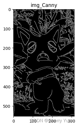
坎尼算子(Canny)
Canny算子要求在提高边缘敏感性的同时抑制噪声,包括如下三个基本目标:
(1)低错误率。所有边缘都应该被找到,并且不应有虚假响应。
(2)边缘点应被很好地定位。检测地边缘点要尽可能地接近实际边缘地中心。有检测算子标记为边缘一点和真实边缘的中心之间的距离应该最小。
(3)单一边缘有且只有一个准确的响应,并尽可能地抑制虚假边缘。即:对于每一个真实的边缘点,检测算子应只返回一个点。真实边缘周围的局部最大数应是最小的。这意味着检测算子不应识别只存在单个边缘点的多个边缘像素。
那么,Canny边缘检测算法的基本步骤:
(1)使用高斯滤波器平滑图像。
G
(
x
,
y
)
=
e
−
x
2
+
y
2
2
σ
2
G(x,y)=e^{-\frac{x^2+y^2}{2{\sigma}^2}}
G(x,y)=e−2σ2x2+y2
(2)用一阶有限差分计算梯度和方向。
(3)对梯度幅值进行非极大值机制(NMS)。
(4)通过双阈值处理和连通性分析检测和连接边缘。
import cv2
import numpy as np
from matplotlib import pyplot as plt
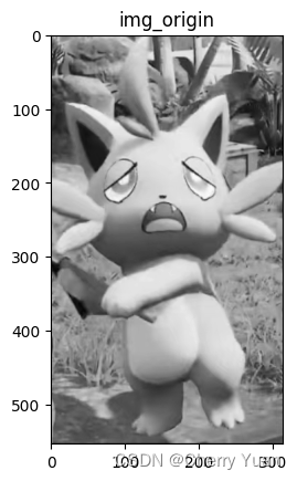
img = cv2.imread("go_work.jpg",flags=0) #读出的图像转化为灰度图
plt.title("img_origin")
plt.imshow(img,cmap="gray")
plt.show()
img_Canny = cv2.Canny(img,threshold1=50,threshold2=150)
plt.title("img_Canny")
plt.imshow(img_Canny,cmap="gray")
plt.show()
结语
你不干


 8130
8130


 被折叠的 条评论
为什么被折叠?
被折叠的 条评论
为什么被折叠?
 到【灌水乐园】发言


