


文章目录
前言
之前所述低通滤波算法的作用是平滑图像以降低噪声,本质上是对图像不同邻域内的像素值进行加权求和、求平均、求中值等等,目的只有一个,就是让相邻像素之间的过度更加平滑些。
锐化,通俗地讲就是突出图像的边缘部分。为了与平滑降噪的低通算法相对应,我们称之为高通滤波。那么高通滤波的基础模型又是从何而来呢?
一、高通滤波的数学定义
我们可以想象一下,图像的像素值在不同邻域内都有其变化的过程,我还是拿二哈先生开刀吧!
import numpy as np
import matplotlib.pyplot as plt
from PIL import Image

#先考虑对灰度图尝试一下吧
img = Image.open("guapi.png")

img_gray = img.convert("L")

plt.title("erha_gray")
plt.imshow(img_gray,cmap="gray")
plt.show()

img_arr = np.array(img_gray)
h,w = img_arr.shape

img_new = np.zeros((h,w))

#这里我打算分两种情况进行简单的高通滤波。

#第一种:水平滤波。所选矩阵为[[1 -1] [0 0]]
filter = np.matrix([[1,-1],[0,0]])
for i in range(1,h-1):
    for j in range(1,w-1):
        img_new[i,j] = np.sum(np.multiply(img_arr[i-1:i+1,j-1:j+1],filter))

img_new = np.uint8(img_new)

plt.title("erha_new1")
plt.imshow(img_new,cmap="gray")
plt.show()

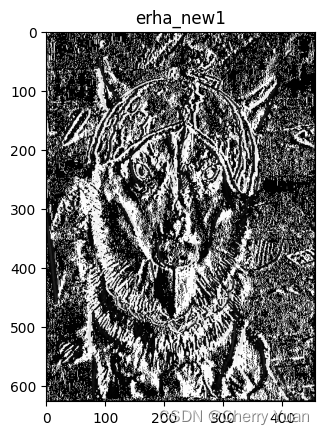
我们会发现,整个图像变得颇有些素描风格了。
import numpy as np
import matplotlib.pyplot as plt
from PIL import Image

#先考虑对灰度图尝试一下吧
img = Image.open("guapi.png")

plt.title("erha_origin")
plt.imshow(img,cmap="brg")
plt.show()

img_arr = np.array(img)
h,w,channels = img_arr.shape

img_new_color = np.zeros((h,w,channels))


filter = np.matrix([[1,-1],[0,0]])
for ch in range(channels):
    for i in range(1,h-1):
        for j in range(1,w-1):
            img_new_color[i,j,ch] = np.sum(np.multiply(img_arr[i-1:i+1,j-1:j+1,ch],filter))

img_new = np.uint8(img_new_color)

plt.title("erha_new_color")
plt.imshow(img_new_color,cmap="brg")
plt.show()

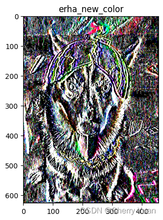
如果是处理彩色图,那就完全没必要了,因为高通滤波的目的是获取边缘信息,我们只要拿到清晰可见的轮廓即可。而且,如我们所见,彩色图经过简单的过滤后,颜色信息其实已经严重失真了。所以,接下来我们统一使用灰色图进行高通滤波。
我们会发现所采用的滤波核是一个特殊的算子
[
1
−
1
0
0
]
\begin{bmatrix} 1&-1\\0&0 \end{bmatrix}
[10−10],而且过滤之后的图像有明显的纵向线,这是为什么呢?不着急,我们再看看瓜皮二哈的垂直高通滤波。
import numpy as np
import matplotlib.pyplot as plt
from PIL import Image
#先考虑对灰度图尝试一下吧
img = Image.open("guapi.png")
img_gray = img.convert("L")
plt.title("erha_gray")
plt.imshow(img_gray,cmap="gray")
plt.show()
img_arr = np.array(img_gray)
h,w = img_arr.shape
img_new2 = np.zeros((h,w))
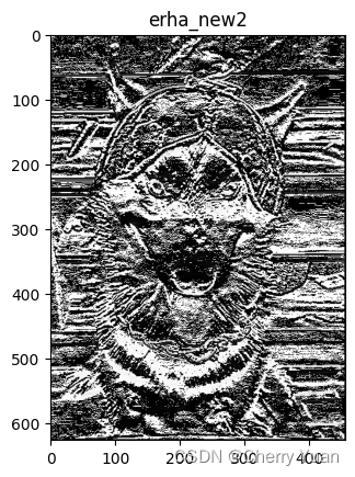
#第二种:垂直滤波。所选矩阵为[[1 0] [-1 0]]
filter2 = np.matrix([[1,0],[-1,0]])
for i in range(1,h-1):
for j in range(1,w-1):
img_new2[i,j] = np.sum(np.multiply(img_arr[i-1:i+1,j-1:j+1],filter2))
img_new2 = np.uint8(img_new2)
plt.title("erha_new2")
plt.imshow(img_new2,cmap="gray")
plt.show()
print(filter2)

[[ 1  0]
 [-1  0]]
现在我们发现原图经过
[
1
0
−
1
0
]
\begin{bmatrix} 1&0\\-1&0 \end{bmatrix}
[1−100]这样垂直方向的高通滤波所产生的新图,里面有一堆横向线。
我们首先需要记住一点,就是水平滤波检测纵向边缘,而垂直滤波检测横向边缘。
关于高通滤波的数学定义,我们可以先考虑图像的横向与纵向像素信息。如果有一张形状为(10,10)的灰度图像,第一行的像素值分别是:199,224,255,254,164,100,55,32,64,99,在这一行内,像素信息从左往右先是变大然后变小,最后再变大,这就有些类似于数学里面讲单调性的情形了,单调递增、单调递减、单调递增这种顺序。如此一来,第一行像素变化就存在某一个邻域内的极值点。
在微分学中,极值点的导数值是0,但像素信息是离散的,所以像素变化过程中我们不可能直接对像素值求导,但我们可以计算横向或者纵向上的像素变化情况。这里就需要引入函数的一阶导数原理公式了。
∂
f
∂
x
=
f
(
x
+
1
)
−
f
(
x
)
\frac{\partial{f}}{\partial{x}}=f(x+1)-f(x)
∂x∂f=f(x+1)−f(x)
模拟连续函数求导的过程,用
f
(
x
+
1
)
f(x+1)
f(x+1)与
f
(
x
)
f(x)
f(x)分别表示
2
×
2
2\times 2
2×2的邻域内水平方向的两个像素值,他们之间相减可以得出该邻域内水平方向的像素的差异,如果颜色相近,结果就接近0,对应的颜色就是接近黑色;如果不相近,结果就为非零值。
我们通过肉眼区分一张图片中的事物,最直观的是通过图像里的颜色信息,一般来说,我们正常遇到的图片都是很好区分的。当然也有一些图片,就算是人类,也很难很快找到图片中的事物,比如迷彩服、变色龙这些。
也就是说,我们正常使用的图像当中,事物的颜色信息会与其周围的环境颜色有很明显的界限。这些图像的灰度图,其事物边缘(轮廓)周围,像素值变化得会特别快,像素值会在边缘出现极值。
这里先画一张简单的黑白图,大家可以看看为什么水平滤波检测纵向边缘,垂直滤波检测横向边缘了。
import numpy as np
import matplotlib.pyplot as plt
from PIL import Image

img = np.ones((100,100,3))*255


for ch in range(3):
    for i in range(20,79):
        for j in range(20,79):
            img[i,j,ch] = 0

img_gray = img[:,:,0] * 0.299 + img[:,:,1] * 0.587 + img[:,:,2] * 0.114
plt.title("img_gray")
plt.imshow(img_gray,cmap="gray")
plt.show()


img_new = np.zeros((100,100))


#第一种:水平滤波。所选矩阵为[[1 -1] [0 0]]
filter = np.matrix([[1,-1],[0,0]])
for i in range(1,99):
    for j in range(1,99):
        img_new[i,j] = np.sum(np.multiply(img_gray[i-1:i+1,j-1:j+1],filter))

img_new = np.uint8(img_new)

plt.title("img_horizon")
plt.imshow(img_new,cmap="gray")
plt.show()
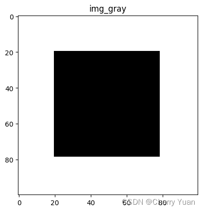
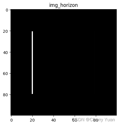
很明显,水平滤波的结果是检测纵向边缘的,但为什么只有一个纵向边缘呢,原因很简单,因为我们只是单纯的
f
(
x
+
1
)
−
f
(
x
)
f(x+1)-f(x)
f(x+1)−f(x),如果差值为负,作为像素值是肯定不行的,所以差值为负的部分默认为黑色了。
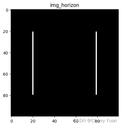
因此,我们需要注意,一阶导求像素变化时的差值是要取绝对值的。我再加一个绝对值看看。
import numpy as np
import matplotlib.pyplot as plt
from PIL import Image

img = np.ones((100,100,3))*255


for ch in range(3):
    for i in range(20,79):
        for j in range(20,79):
            img[i,j,ch] = 0

img_gray = img[:,:,0] * 0.299 + img[:,:,1] * 0.587 + img[:,:,2] * 0.114
plt.title("img_gray")
plt.imshow(img_gray,cmap="gray")
plt.show()


img_new = np.zeros((100,100))


#第一种:水平滤波。所选矩阵为[[1 -1] [0 0]]
filter = np.matrix([[1,-1],[0,0]])
for i in range(1,99):
    for j in range(1,99):
        img_new[i,j] = abs(np.sum(np.multiply(img_gray[i-1:i+1,j-1:j+1],filter)))

img_new = np.uint8(img_new)

plt.title("img_horizon")
plt.imshow(img_new,cmap="gray")
plt.show()

我们再试试垂直滤波的效果。
import numpy as np
import matplotlib.pyplot as plt
from PIL import Image

img = np.ones((100,100,3))*255


for ch in range(3):
    for i in range(20,79):
        for j in range(20,79):
            img[i,j,ch] = 0

img_gray = img[:,:,0] * 0.299 + img[:,:,1] * 0.587 + img[:,:,2] * 0.114
plt.title("img_gray")
plt.imshow(img_gray,cmap="gray")
plt.show()


img_new = np.zeros((100,100))


#第二种:垂直滤波。所选矩阵为[[1 0] [-1 0]]
filter2 = np.matrix([[1,0],[-1,0]])
for i in range(1,99):
    for j in range(1,99):
        img_new[i,j] = abs(np.sum(np.multiply(img_gray[i-1:i+1,j-1:j+1],filter2)))

img_new = np.uint8(img_new)

plt.title("img_horizon")
plt.imshow(img_new,cmap="gray")
plt.show()


其实,用一阶导的差分法表示图像灰度值的变化,其思路来源于函数的泰勒展开式,感兴趣的伙计们可以去了解一下泰勒展开式、高阶导数与图像灰度的联系。
使用二阶导的方法能够更加细粒度地展示图像灰度值得变化。我们先看看一阶导数相关地高通滤波。
二、一阶导(梯度)算法
首先,我们需要注意,这里提到的一阶导数锐化算法,实质上是梯度,而不是一阶导。但如果你还记得高等数学里的知识点,你应该知道,梯度表示函数在某点处最大的变化率,它是由函数的一阶偏导与方向向量运算的来的。
一阶导算子大致如下:
∇
f
=
(
∂
f
∂
x
)
2
+
(
∂
f
∂
y
)
2
=
[
f
(
x
+
1
)
−
f
(
x
)
]
2
+
[
f
(
y
+
1
)
−
f
(
y
)
]
2
\nabla{f}=\sqrt{(\frac{\partial{f}}{\partial{x}})^2+(\frac{\partial{f}}{\partial{y}})^2}=\sqrt{[f(x+1)-f(x)]^2+[f(y+1)-f(y)]^2}
∇f=(∂x∂f)2+(∂y∂f)2=[f(x+1)−f(x)]2+[f(y+1)−f(y)]2
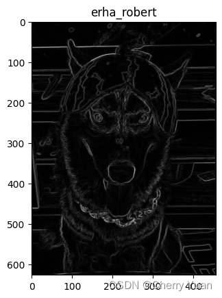
1.罗伯特算子
根据冈萨雷斯的《数字图像处理》第四版可知,罗伯特算子为一个交叉梯度算子,它的形状大致如下。
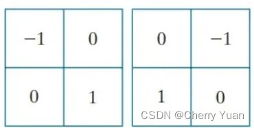
很明显,罗伯特交叉梯度算子具有两个核!假设我们选取图像中的一个 3 × 3 3\times3 3×3的区域,作为滤波器进行运算的一部分。
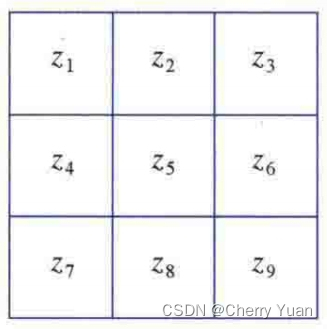
使用罗伯特算子,那我们会得到形如 g x = ( z 9 − z 5 ) g_x=(z_9-z_5) gx=(z9−z5)和 g y = ( z 8 − z 6 ) g_y=(z_8-z_6) gy=(z8−z6)这样的一阶导。根据一阶导算子的原理公式可将罗伯特算子公式所得的滤波算子写成: M ( x , y ) = [ ( z 9 − z 5 ) 2 + ( z 8 − z 6 ) 2 ] 1 2 M(x,y)=[(z_9-z_5)^2+(z_8-z_6)^2]^{\frac{1}{2}} M(x,y)=[(z9−z5)2+(z8−z6)2]21
有时公式可以简化为: M ( x , y ) ≈ ∣ z 9 − z 5 ∣ + ∣ z 8 − z 6 ∣ M(x,y)\approx|z_9-z_5|+|z_8-z_6| M(x,y)≈∣z9−z5∣+∣z8−z6∣
但是近似的取绝对值,有时效果并不是很好,所以我们尽可能选择原公式的方法。
其中
M
(
x
,
y
)
M(x,y)
M(x,y)就是与原图像大小相同的图像,是经过算子不断滤波运算得到的结果。那么下面我还是拿二哈开刀试试吧!
#近似等于的公式
import numpy as np
import matplotlib.pyplot as plt
from PIL import Image

img = Image.open("guapi.png")

img_gray = img.convert("L")

plt.title("erha_gray")
plt.imshow(img_gray,cmap="gray")
plt.show()

img_arr = np.array(img_gray)
h,w = img_arr.shape

img_robert = np.zeros((h,w))

filter_robert_x = np.matrix([[-1,0],[0,1]])
filter_robert_y = np.matrix([[0,-1],[1,0]])
for i in range(1,h-1):
    for j in range(1,w-1):
        img_robert[i,j] = abs(np.sum(np.multiply(img_arr[i-1:i+1,j-1:j+1],filter_robert_x))) + abs(np.sum(np.multiply(img_arr[i-1:i+1,j-1:j+1],filter_robert_y)))

img_robert = np.uint8(img_robert)

plt.title("erha_robert")
plt.imshow(img_robert,cmap="gray")
plt.show()

#原公式
import numpy as np
import matplotlib.pyplot as plt
from PIL import Image
import math

img = Image.open("guapi.png")

img_gray = img.convert("L")

plt.title("erha_gray")
plt.imshow(img_gray,cmap="gray")
plt.show()

img_arr = np.array(img_gray)
h,w = img_arr.shape

img_robert = np.zeros((h,w))

filter_robert_x = np.matrix([[-1,0],[0,1]])
filter_robert_y = np.matrix([[0,-1],[1,0]])
for i in range(1,h-1):
    for j in range(1,w-1):
        img_robert[i,j] = math.sqrt((np.sum(np.multiply(img_arr[i-1:i+1,j-1:j+1],filter_robert_x))) ** 2 + (np.sum(np.multiply(img_arr[i-1:i+1,j-1:j+1],filter_robert_y))) ** 2)

img_robert = np.uint8(img_robert)

plt.title("erha_robert")
plt.imshow(img_robert,cmap="gray")
plt.show()


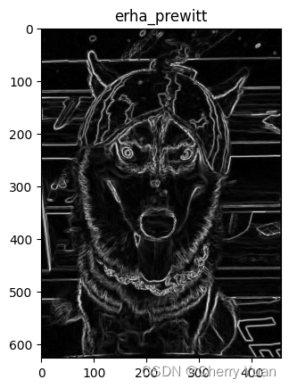
2、Prewitt算子
在学习Sobel算子之前我们先看看它的前身:
K
x
[
−
1
0
1
−
1
0
1
−
1
0
1
]
K_x\begin{bmatrix}-1&0&1\\-1&0&1\\-1&0&1\end{bmatrix}
Kx
−1−1−1000111
K
y
=
[
−
1
−
1
−
1
0
0
0
1
1
1
]
K_y=\begin{bmatrix}-1&-1&-1\\0&0&0\\1&1&1\end{bmatrix}
Ky=
−101−101−101
#Prewitt
import numpy as np
import matplotlib.pyplot as plt
from PIL import Image
import math

img = Image.open("guapi.png")

img_gray = img.convert("L")

plt.title("erha_gray")
plt.imshow(img_gray,cmap="gray")
plt.show()

img_arr = np.array(img_gray)
h,w = img_arr.shape

img_prewitt = np.zeros((h,w))

filter_prewitt_x = np.matrix([[-1,0,1],[-1,0,1],[-1,0,1]])
filter_prewitt_y = np.matrix([[-1,-1,-1],[0,0,0],[1,1,1]])

for i in range(1,h-1):
    for j in range(1,w-1):
        img_prewitt[i,j] = math.sqrt((np.sum(np.multiply(img_arr[i-1:i+2,j-1:j+2],filter_prewitt_x))) ** 2 + (np.sum(np.multiply(img_arr[i-1:i+2,j-1:j+2],filter_prewitt_y))) ** 2)

img_prewitt = np.uint8(img_prewitt)

plt.title("erha_prewitt")
plt.imshow(img_prewitt,cmap="gray")
plt.show()

3.Sobel算子
Sobel算子就是常见得锐化算子了。
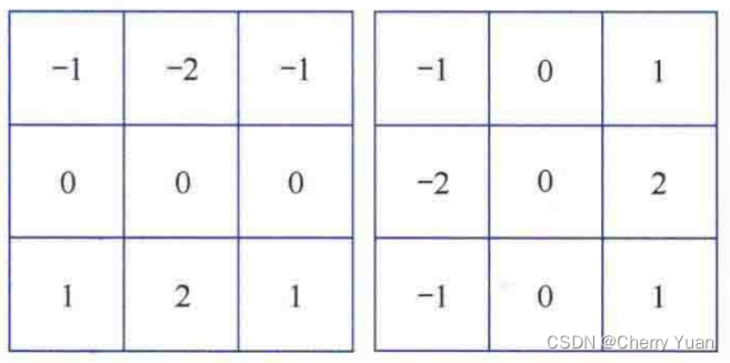
与Robert算子一样,Sobel也是一个交叉梯度算子,但我们习惯于使用奇数大小的核。Sobel两个方向的一阶导表示分别是: g x = ∂ f ∂ x = ( z 7 + 2 z 8 + z 9 ) − ( z 1 + 2 z 2 + z 3 ) g_x=\frac{\partial{f}}{\partial{x}}=(z_7+2z_8+z_9)-(z_1+2z_2+z_3) gx=∂x∂f=(z7+2z8+z9)−(z1+2z2+z3) g y = ∂ f ∂ y = ( z 3 + 2 z 6 + z 9 ) − ( z 1 + 2 z 4 + z 7 ) g_y=\frac{\partial{f}}{\partial{y}}=(z_3+2z_6+z_9)-(z_1+2z_4+z_7) gy=∂y∂f=(z3+2z6+z9)−(z1+2z4+z7)
相应的 M ( x , y ) M(x,y) M(x,y)(梯度幅度)公式如下: M ( x , y ) = [ g x 2 + g y 2 ] = [ [ ( z 7 + 2 z 8 + z 9 ) − ( z 1 + 2 z 2 + z 3 ) ] 2 + [ ( z 3 + 2 z 6 + z 9 ) − ( z 1 + 2 z 4 + z 7 ) ] 2 ] 1 2 M(x,y)=[{g_x}^2+{g_y}^2]=[[(z_7+2z_8+z_9)-(z_1+2z_2+z_3)]^2+[(z_3+2z_6+z_9)-(z_1+2z_4+z_7)]^2]^{\frac{1}{2}} M(x,y)=[gx2+gy2]=[[(z7+2z8+z9)−(z1+2z2+z3)]2+[(z3+2z6+z9)−(z1+2z4+z7)]2]21
Sobel算子的中心系数是2的原因是,强调中心的重要程度,集合了高斯平滑。
#Sobel算子原公式
import numpy as np
import matplotlib.pyplot as plt
from PIL import Image
import math

img = Image.open("guapi.png")

img_gray = img.convert("L")

plt.title("erha_gray")
plt.imshow(img_gray,cmap="gray")
plt.show()

img_arr = np.array(img_gray)
h,w = img_arr.shape

img_sobel = np.zeros((h,w))

filter_sobel_x = np.matrix([[-1,0,1],[-2,0,2],[-1,0,1]])
filter_sobel_y = np.matrix([[-1,-2,-1],[0,0,0],[1,2,1]])

for i in range(1,h-1):
    for j in range(1,w-1):
        img_sobel[i,j] = math.sqrt((np.sum(np.multiply(img_arr[i-1:i+2,j-1:j+2],filter_sobel_x))) ** 2 + (np.sum(np.multiply(img_arr[i-1:i+2,j-1:j+2],filter_sobel_y))) ** 2)

img_sobel = np.uint8(img_sobel)

plt.title("erha_Sobel")
plt.imshow(img_sobel,cmap="gray")
plt.show()


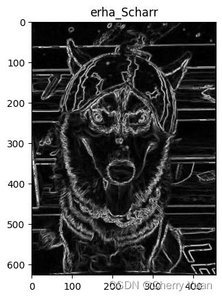
4、Scharr算子
Scharr算子又是一个 3 × 3 3\times3 3×3大小的一阶导核的变种:
K x = [ − 3 0 3 − 10 0 − 10 − 3 0 3 ] K_x=\begin{bmatrix} -3&0&3\\-10&0&-10\\-3&0&3 \end{bmatrix} Kx= −3−10−30003−103
K y [ − 3 − 10 − 3 0 0 0 3 10 3 ] K_y\begin{bmatrix} -3&-10&-3\\0&0&0\\3&10&3 \end{bmatrix} Ky −303−10010−303
#Scharr算子
import numpy as np
import matplotlib.pyplot as plt
from PIL import Image
import math

img = Image.open("guapi.png")

img_gray = img.convert("L")

plt.title("erha_gray")
plt.imshow(img_gray,cmap="gray")
plt.show()

img_arr = np.array(img_gray)
h,w = img_arr.shape

img_scharr = np.zeros((h,w))

filter_scharr_x = np.matrix([[-3,0,3],[-10,0,10],[-3,0,3]])
filter_scharr_y = np.matrix([[-3,-10,-3],[0,0,0],[3,10,3]])

for i in range(1,h-1):
    for j in range(1,w-1):
        img_scharr[i,j] = math.sqrt((np.sum(np.multiply(img_arr[i-1:i+2,j-1:j+2],filter_scharr_x))) ** 2 + (np.sum(np.multiply(img_arr[i-1:i+2,j-1:j+2],filter_scharr_y))) ** 2)

img_scharr = np.uint8(img_sobel)

plt.title("erha_Scharr")
plt.imshow(img_scharr,cmap="gray")
plt.show()

三、二阶导(梯度)算法
与一阶导数相比,二阶导数可增强更精细的细节,因此适合锐化图像的一些理想特性。另外,与实现一阶导数相比,实现二阶导数所需的运算量更少。
拉普拉斯(Laplacian)算子
首先,熟悉一下公式吧! ∇ 2 f ( x , y ) = ∂ 2 f ∂ x 2 + ∂ 2 f ∂ y 2 \nabla^2{f(x,y)}=\frac{\partial^2{f}}{\partial{x^2}}+\frac{\partial^2{f}}{\partial{y^2}} ∇2f(x,y)=∂x2∂2f+∂y2∂2f
∂ 2 f ∂ x 2 = f ( x + 1 , y ) + f ( x − 1 , y ) − 2 f ( x , y ) \frac{\partial^2{f}}{\partial{x^2}}=f(x+1,y)+f(x-1,y)-2f(x,y) ∂x2∂2f=f(x+1,y)+f(x−1,y)−2f(x,y)
∂ 2 f ∂ y 2 = f ( x , y + 1 ) + f ( x , y − 1 ) − 2 f ( x , y ) \frac{\partial^2{f}}{\partial{y^2}}=f(x,y+1)+f(x,y-1)-2f(x,y) ∂y2∂2f=f(x,y+1)+f(x,y−1)−2f(x,y)
离散拉普拉斯的公式: ∇ 2 f ( x , y ) = f ( x + 1 , y ) + f ( x − 1 , y ) + f ( x , y + 1 ) + f ( x , y − 1 ) − 4 f ( x , y ) \nabla^2{f(x,y)}=f(x+1,y)+f(x-1,y)+f(x,y+1)+f(x,y-1)-4f(x,y) ∇2f(x,y)=f(x+1,y)+f(x−1,y)+f(x,y+1)+f(x,y−1)−4f(x,y)
终式: g ( x , y ) = f ( x , y ) + c [ ∇ 2 f ( x , y ) ] g(x,y)=f(x,y)+c[\nabla^2{f(x,y)}] g(x,y)=f(x,y)+c[∇2f(x,y)]
f ( x , y ) f(x,y) f(x,y)和 g ( x , y ) g(x,y) g(x,y)分别表示输入图像和锐化后的图像。
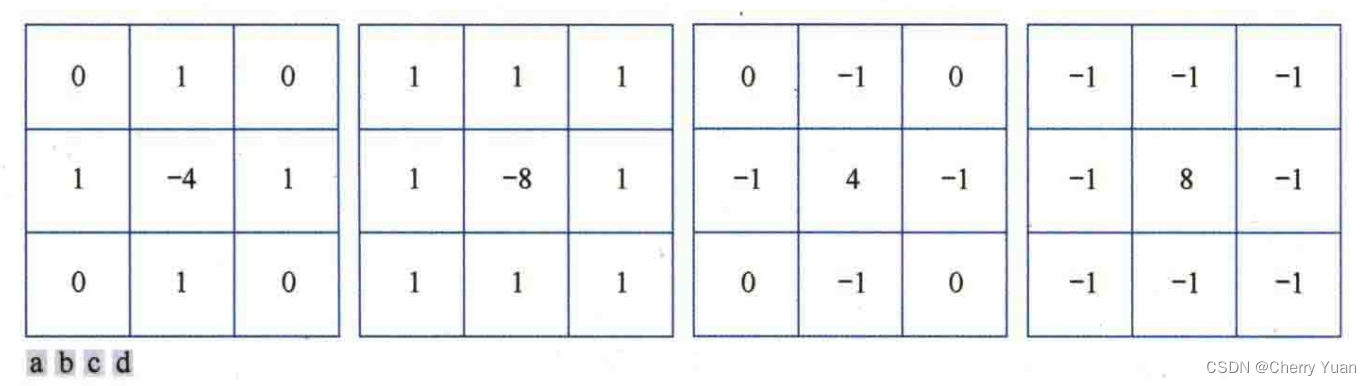
如图,图a是离散拉普拉斯核,图b是实现其中包含对角项的扩展式的核。如果我们选择a、b这两种拉普拉斯核,那么终式中的系数c就是1,如果我们选择c、d两种核,那么系数c就是-1。
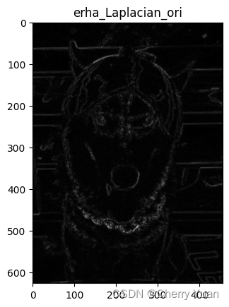
#离散拉普拉斯核
import numpy as np
import matplotlib.pyplot as plt
from PIL import Image
import math
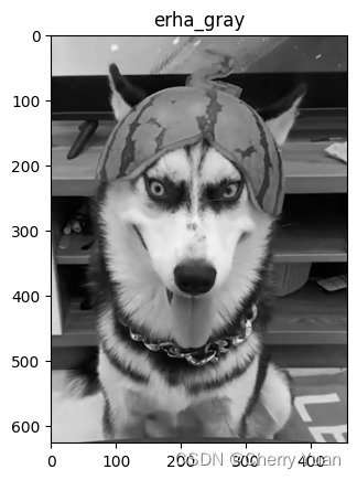
img = Image.open("guapi.png")
img_gray = img.convert("L")
plt.title("erha_gray")
plt.imshow(img_gray,cmap="gray")
plt.show()
img_arr = np.array(img_gray)
h,w = img_arr.shape
img_laplacian_ori = np.zeros((h,w))
laplacian_ori = np.zeros((h,w))
filter_laplacian_ori = np.matrix([[0,1,0],[1,-4,1],[0,1,0]])
for i in range(1,h-1):
for j in range(1,w-1):
laplacian_ori[i,j] = abs(np.sum(np.multiply(img_arr[i-1:i+2,j-1:j+2],filter_laplacian_ori)))
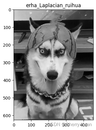
img_laplacian_ori = img_arr + laplacian_ori
laplacian_ori = np.uint8(laplacian_ori)
img_laplacian_ori = np.uint8(img_laplacian_ori)
plt.title("erha_Laplacian_ori")
plt.imshow(laplacian_ori,cmap="gray")
plt.show()
plt.title("erha_Laplacian_ruihua")
plt.imshow(img_laplacian_ori,cmap="gray")
plt.show()
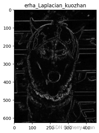
#对角项扩展式拉普拉斯核
import numpy as np
import matplotlib.pyplot as plt
from PIL import Image
import math
img = Image.open("guapi.png")
img_gray = img.convert("L")
plt.title("erha_gray")
plt.imshow(img_gray,cmap="gray")
plt.show()
img_arr = np.array(img_gray)
h,w = img_arr.shape
img_laplacian_kuozhan = np.zeros((h,w))
laplacian_kuozhan = np.zeros((h,w))
filter_laplacian_kuozhan = np.matrix([[1,1,1],[1,-8,1],[1,1,1]])
for i in range(1,h-1):
for j in range(1,w-1):
laplacian_kuozhan[i,j] = abs(np.sum(np.multiply(img_arr[i-1:i+2,j-1:j+2],filter_laplacian_kuozhan)))
img_laplacian_kuozhan = img_arr + laplacian_kuozhan
laplacian_kuozhan = np.uint8(laplacian_kuozhan)
img_laplacian_kuozhan = np.uint8(img_laplacian_kuozhan)
plt.title("erha_Laplacian_kuozhan")
plt.imshow(laplacian_kuozhan,cmap="gray")
plt.show()
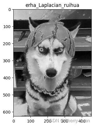
plt.title("erha_Laplacian_ruihua")
plt.imshow(img_laplacian_kuozhan,cmap="gray")
plt.show()

四、钝化掩蔽核高提升滤波
钝化掩蔽,是从原图中减去一幅(平滑后)的图像,具体步骤如下:
1.模糊原图像。
2.从原图像减去模糊后的图像(产生的差成为模板)。
3.将模板与原图像相加。
令 f ‾ ( x , y ) \overline{f}(x,y) f(x,y)表示模糊后的图像,公式形式的模板为: g m a s k ( x , y ) = f ( x , y ) − f ‾ ( x , y ) g_{mask}(x,y)=f(x,y)- \overline{f}(x,y) gmask(x,y)=f(x,y)−f(x,y)
然后,将加权后的模板与原图像相加: g ( x , y ) = f ( x , y ) + k g m a s k ( x , y ) g(x,y)=f(x,y)+kg_{mask}(x,y) g(x,y)=f(x,y)+kgmask(x,y)
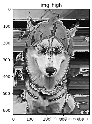
为了不失一般性,式中包含了一个权值 k ( k ≥ 0 ) k(k\geq0) k(k≥0)。 k = 1 k=1 k=1时,它是钝化掩蔽。 k > 1 k>1 k>1时,这个过程称为高提升滤波。若选择 k < 1 k<1 k<1则可以减少钝化膜板的贡献。
1.钝化掩蔽
接下来,我们先试着使用高斯低通滤波器来模糊图像。
#高斯滤波器
import numpy as np
import matplotlib.pyplot as plt
from PIL import Image


#所选图片为彩色图,维度为3,通道数为3
image = Image.open("guapi.png")
image = np.array(image)
h_img,w_img,ch = image.shape
# print(image)

plt.title("image_origin")
plt.imshow(image,cmap="brg")
plt.show()

#创建相关运算二维核,而且一般来说,滤波器核的大小都是奇数。
def creat_filter(ksize,std):

    filter = np.ones((ksize,ksize))

    sigma = std

    for x in range(ksize):
        for y in range(ksize):
            filter[x,y] = filter[x,y] * np.exp(((x - (ksize - 1)/2) ** 2 + (y - (ksize - 1)/2) ** 2) * (-1)/(sigma ** 2 * 2)) / (2 * np.pi * sigma ** 2)
    return filter

#边界扩充:填充,相关运算和卷积运算对图像边界点进行特殊处理时,需要适当扩充图像边界。默认填充0,代表黑色。其中padding为填充0的圈数。
#为了使经过滤波器核输出的图像大小和原图一致,本次实验选择高和宽都填充两层。即:padding = h_f - 1。(padding = w_f - 1)
#注意此处滤波器核大小是奇数。

def padding_image_3d(image,h_f,w_f):
    h_img,w_img,ch = image.shape
    h_new,w_new = h_img + h_f - 1,w_img + w_f - 1
    image_padding = np.zeros((h_new,w_new,ch))
    for k in range(ch):
        for i in range(h_img):
            for j in range(w_img):
                image_padding[i + int((h_f-1)/2),j + int((w_f-1)/2),k] = image[i,j,k]
    return image_padding

#空间卷积运算,注意:这里的d一定是偶数
def convolution_operation(image,filter):
    h_img,w_img,ch = image.shape
    h_f,w_f = filter.shape
    filter_convolution = np.flip(filter)#卷积运算所需二维核是对相关运算二维核的翻转。
    image_out = np.zeros((h_img,w_img,ch))
    image_padding = padding_image_3d(image,h_f,w_f)

    for k in range(ch):
        for i in range(h_img):
            for j in range(w_img):
                image_out[i,j,k] = np.sum(np.multiply(filter_convolution[:,:],image_padding[i:i+h_f,j:j+w_f,k]))
    return image_out

def draw_convolution(ksize,std):
    image_convolution = convolution_operation(image,creat_filter(ksize,std))
    image_out = np.uint8(image_convolution)

    plt.title("image_Gaussian")
    plt.imshow(image_out,cmap="brg")
    plt.show()

if __name__ == "__main__":
    draw_convolution(ksize=31,std=5)

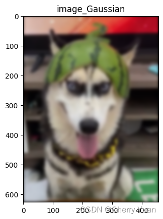
如上所述,所使用的高斯核时
31
×
31
31\times31
31×31的大小,标准差为5。接下来我要开始用原图减去模糊图了。
#钝化模板
import numpy as np
import matplotlib.pyplot as plt
from PIL import Image


#所选图片为彩色图,维度为3,通道数为3
image = Image.open("guapi.png")
image = np.array(image)
h_img,w_img,ch = image.shape
# print(image)

plt.title("image_origin")
plt.imshow(image,cmap="brg")
plt.show()

#创建相关运算二维核,而且一般来说,滤波器核的大小都是奇数。
def creat_filter(ksize,std):

    filter = np.ones((ksize,ksize))

    sigma = std

    for x in range(ksize):
        for y in range(ksize):
            filter[x,y] = filter[x,y] * np.exp(((x - (ksize - 1)/2) ** 2 + (y - (ksize - 1)/2) ** 2) * (-1)/(sigma ** 2 * 2)) / (2 * np.pi * sigma ** 2)
    return filter

#边界扩充:填充,相关运算和卷积运算对图像边界点进行特殊处理时,需要适当扩充图像边界。默认填充0,代表黑色。其中padding为填充0的圈数。
#为了使经过滤波器核输出的图像大小和原图一致,本次实验选择高和宽都填充两层。即:padding = h_f - 1。(padding = w_f - 1)
#注意此处滤波器核大小是奇数。

def padding_image_3d(image,h_f,w_f):
    h_img,w_img,ch = image.shape
    h_new,w_new = h_img + h_f - 1,w_img + w_f - 1
    image_padding = np.zeros((h_new,w_new,ch))
    for k in range(ch):
        for i in range(h_img):
            for j in range(w_img):
                image_padding[i + int((h_f-1)/2),j + int((w_f-1)/2),k] = image[i,j,k]
    return image_padding

#空间卷积运算,注意:这里的d一定是偶数
def convolution_operation(image,filter):
    h_img,w_img,ch = image.shape
    h_f,w_f = filter.shape
    filter_convolution = np.flip(filter)#卷积运算所需二维核是对相关运算二维核的翻转。
    image_out = np.zeros((h_img,w_img,ch))
    image_padding = padding_image_3d(image,h_f,w_f)

    for k in range(ch):
        for i in range(h_img):
            for j in range(w_img):
                image_out[i,j,k] = np.sum(np.multiply(filter_convolution[:,:],image_padding[i:i+h_f,j:j+w_f,k]))
    return image_out

def draw_convolution(ksize,std):
    image_convolution = convolution_operation(image,creat_filter(ksize,std))

    #原图减去模糊图
    image_mask = image - image_convolution

    image_mask = np.uint8(image_mask)

    plt.title("image_dunhua")
    plt.imshow(image_mask,cmap="brg")
    plt.show()

if __name__ == "__main__":
    draw_convolution(ksize=31,std=5)

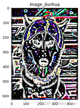
最后一步,钝化模板加上原图
#钝化模板+原图
import numpy as np
import matplotlib.pyplot as plt
from PIL import Image


#所选图片为彩色图,维度为3,通道数为3
image = Image.open("guapi.png")
image = np.array(image)
h_img,w_img,ch = image.shape
# print(image)

plt.title("image_origin")
plt.imshow(image,cmap="brg")
plt.show()

#创建相关运算二维核,而且一般来说,滤波器核的大小都是奇数。
def creat_filter(ksize,std):

    filter = np.ones((ksize,ksize))

    sigma = std

    for x in range(ksize):
        for y in range(ksize):
            filter[x,y] = filter[x,y] * np.exp(((x - (ksize - 1)/2) ** 2 + (y - (ksize - 1)/2) ** 2) * (-1)/(sigma ** 2 * 2)) / (2 * np.pi * sigma ** 2)
    return filter

#边界扩充:填充,相关运算和卷积运算对图像边界点进行特殊处理时,需要适当扩充图像边界。默认填充0,代表黑色。其中padding为填充0的圈数。
#为了使经过滤波器核输出的图像大小和原图一致,本次实验选择高和宽都填充两层。即:padding = h_f - 1。(padding = w_f - 1)
#注意此处滤波器核大小是奇数。

def padding_image_3d(image,h_f,w_f):
    h_img,w_img,ch = image.shape
    h_new,w_new = h_img + h_f - 1,w_img + w_f - 1
    image_padding = np.zeros((h_new,w_new,ch))
    for k in range(ch):
        for i in range(h_img):
            for j in range(w_img):
                image_padding[i + int((h_f-1)/2),j + int((w_f-1)/2),k] = image[i,j,k]
    return image_padding


#空间卷积运算,注意:这里的d一定是偶数
def convolution_operation(image,filter):
    h_img,w_img,ch = image.shape
    h_f,w_f = filter.shape
    filter_convolution = np.flip(filter)#卷积运算所需二维核是对相关运算二维核的翻转。
    image_out = np.zeros((h_img,w_img,ch))
    image_padding = padding_image_3d(image,h_f,w_f)

    for k in range(ch):
        for i in range(h_img):
            for j in range(w_img):
                image_out[i,j,k] = np.sum(np.multiply(filter_convolution[:,:],image_padding[i:i+h_f,j:j+w_f,k]))
    return image_out

def draw_convolution(ksize,std):
    image_convolution = convolution_operation(image,creat_filter(ksize,std))

    #原图减去模糊图
    image_mask = image - image_convolution

    #钝化模板+原图
    image_out = image + image_mask

    image_out = np.uint8(image_out)

    plt.title("image_dunhua_yanbi")
    plt.imshow(image_out,cmap="brg")
    plt.show()

if __name__ == "__main__":
    draw_convolution(ksize=31,std=5)

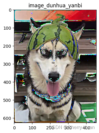
完了,狗子变得贼帅!!!
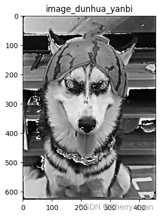
先前的例子是彩色图,我们还是用灰度图吧
#钝化模板+原图
import numpy as np
import matplotlib.pyplot as plt
from PIL import Image
#所选图片为彩色图,维度为3,通道数为3
image = Image.open("guapi.png")
image = image.convert("L")
image = np.array(image)
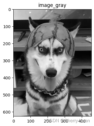
plt.title("image_gray")
plt.imshow(image,cmap="gray")
plt.show()
#创建相关运算二维核,而且一般来说,滤波器核的大小都是奇数。
def creat_filter(ksize,std):
filter = np.ones((ksize,ksize))
sigma = std
for x in range(ksize):
for y in range(ksize):
filter[x,y] = filter[x,y] * np.exp(((x - (ksize - 1)/2) ** 2 + (y - (ksize - 1)/2) ** 2) * (-1)/(sigma ** 2 * 2)) / (2 * np.pi * sigma ** 2)
return filter
#边界扩充:填充,相关运算和卷积运算对图像边界点进行特殊处理时,需要适当扩充图像边界。默认填充0,代表黑色。其中padding为填充0的圈数。
#为了使经过滤波器核输出的图像大小和原图一致,本次实验选择高和宽都填充两层。即:padding = h_f - 1。(padding = w_f - 1)
#注意此处滤波器核大小是奇数。
def padding_image(image,h_f,w_f):
h_img,w_img = image.shape
h_new,w_new = h_img + h_f - 1,w_img + w_f - 1
image_padding = np.zeros((h_new,w_new))
for i in range(h_img):
for j in range(w_img):
image_padding[i + int((h_f-1)/2),j + int((w_f-1)/2)] = image[i,j]
return image_padding
#空间卷积运算,注意:这里的d一定是偶数
def convolution_operation(image,filter):
h_img,w_img= image.shape
h_f,w_f = filter.shape
filter_convolution = np.flip(filter)#卷积运算所需二维核是对相关运算二维核的翻转。
image_out = np.zeros((h_img,w_img))
image_padding = padding_image(image,h_f,w_f)
for i in range(h_img):
for j in range(w_img):
image_out[i,j] = np.sum(np.multiply(filter_convolution[:,:],image_padding[i:i+h_f,j:j+w_f]))
return image_out
def draw_convolution(ksize,std):
image_convolution = convolution_operation(image,creat_filter(ksize,std))
#原图减去模糊图
image_mask = image - image_convolution
#钝化模板+原图
image_out = image + image_mask
image_out = np.uint8(image_out)
plt.title("image_dunhua_yanbi")
plt.imshow(image_out,cmap="gray")
plt.show()
if __name__ == "__main__":
draw_convolution(ksize=31,std=5)

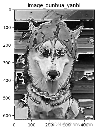
2.高提升滤波
#高提升滤波
import numpy as np
import matplotlib.pyplot as plt
from PIL import Image


#所选图片为彩色图,维度为3,通道数为3
image = Image.open("guapi.png")
image = image.convert("L")
image = np.array(image)

plt.title("image_gray")
plt.imshow(image,cmap="gray")
plt.show()

#创建相关运算二维核,而且一般来说,滤波器核的大小都是奇数。
def creat_filter(ksize,std):

    filter = np.ones((ksize,ksize))

    sigma = std

    for x in range(ksize):
        for y in range(ksize):
            filter[x,y] = filter[x,y] * np.exp(((x - (ksize - 1)/2) ** 2 + (y - (ksize - 1)/2) ** 2) * (-1)/(sigma ** 2 * 2)) / (2 * np.pi * sigma ** 2)
    return filter

#边界扩充:填充,相关运算和卷积运算对图像边界点进行特殊处理时,需要适当扩充图像边界。默认填充0,代表黑色。其中padding为填充0的圈数。
#为了使经过滤波器核输出的图像大小和原图一致,本次实验选择高和宽都填充两层。即:padding = h_f - 1。(padding = w_f - 1)
#注意此处滤波器核大小是奇数。
def padding_image(image,h_f,w_f):
    h_img,w_img = image.shape
    h_new,w_new = h_img + h_f - 1,w_img + w_f - 1
    image_padding = np.zeros((h_new,w_new))
    for i in range(h_img):
        for j in range(w_img):
            image_padding[i + int((h_f-1)/2),j + int((w_f-1)/2)] = image[i,j]
    return image_padding

#空间卷积运算,注意:这里的d一定是偶数
def convolution_operation(image,filter):
    h_img,w_img= image.shape
    h_f,w_f = filter.shape
    filter_convolution = np.flip(filter)#卷积运算所需二维核是对相关运算二维核的翻转。
    image_out = np.zeros((h_img,w_img))
    image_padding = padding_image(image,h_f,w_f)

    for i in range(h_img):
        for j in range(w_img):
            image_out[i,j] = np.sum(np.multiply(filter_convolution[:,:],image_padding[i:i+h_f,j:j+w_f]))
    return image_out

def draw_convolution(ksize,std):
    image_convolution = convolution_operation(image,creat_filter(ksize,std))

    #原图减去模糊图
    image_mask = image - image_convolution

    #钝化模板+原图
    image_out = image + image_mask * 2

    image_out = np.uint8(image_out)

    plt.title("image_dunhua_yanbi")
    plt.imshow(image_out,cmap="gray")
    plt.show()

if __name__ == "__main__":
    draw_convolution(ksize=31,std=5)
3.章节回顾
看到这儿大家可能会疑惑,为什么图像变得怪怪的。其实原因很简单,因为我选择numpy常见的高斯核各像素值是全1的,高斯核利用numpy创建的方式有很多种可能。关于多种可能的高斯滤波器,我在之前的《图像空间低通滤波》博客中已经提到了,感兴趣的伙计们可以自己选择其他类型的高斯核进行钝化掩蔽和高提升。
我还是想延续低通滤波那篇的写法,最后来一个OpenCV的钝化掩蔽和高提升滤波。
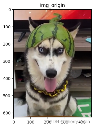
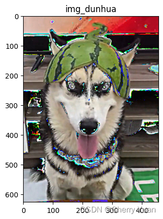
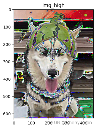
#使用OpenCV库进行二维高斯滤波运算
import cv2
import matplotlib.pyplot as plt
img = cv2.imread("guapi.png")
img = cv2.cvtColor(img,cv2.COLOR_BGR2RGB)
ksize_31 = (31,31)
Gauss_filter31 = cv2.GaussianBlur(img,ksize_31,5)
plt.title("img_origin")
plt.imshow(img,cmap="brg",vmin=0,vmax=255)
plt.show()
plt.title("img_Gauss_filter31")
plt.imshow(Gauss_filter31,cmap="brg",vmin=0,vmax=255)
plt.show()
#钝化模板
image_mask = img - Gauss_filter31
#钝化掩蔽
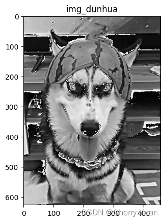
image_dunhua = img + image_mask
#高提升(k=2)
image_high = img + image_mask * 2
plt.title("img_dunhua")
plt.imshow(image_dunhua,cmap="brg",vmin=0,vmax=255)
plt.show()
plt.title("img_high")
plt.imshow(image_high,cmap="brg",vmin=0,vmax=255)
plt.show()

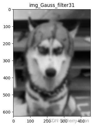
#使用OpenCV库进行二维高斯滤波运算
import cv2
import matplotlib.pyplot as plt

img = cv2.imread("guapi.png")
img = cv2.cvtColor(img,cv2.COLOR_BGR2GRAY)

ksize_31 = (31,31)
Gauss_filter31 = cv2.GaussianBlur(img,ksize_31,5)

plt.title("img_gray")
plt.imshow(img,cmap="gray",vmin=0,vmax=255)
plt.show()

plt.title("img_Gauss_filter31")
plt.imshow(Gauss_filter31,cmap="gray",vmin=0,vmax=255)
plt.show()

#钝化模板
image_mask = img - Gauss_filter31

#钝化掩蔽
image_dunhua = img + image_mask

#高提升(k=2)
image_high = img + image_mask * 2

plt.title("img_dunhua")
plt.imshow(image_dunhua,cmap="gray",vmin=0,vmax=255)
plt.show()

plt.title("img_high")
plt.imshow(image_high,cmap="gray",vmin=0,vmax=255)
plt.show()

五、结语
关于高通滤波的一阶导和二阶导算子及其锐化效果先告一段落,后续关于低通和高通滤波的拓展补充会在接下来的博客创作中体现,尽情期待吧!


 2万+
2万+


 被折叠的 条评论
为什么被折叠?
被折叠的 条评论
为什么被折叠?
 到【灌水乐园】发言


