【Numpy】图像处理——全局阈值处理（二值化）

Cherry Yuan

已于 2024-02-22 17:12:10 修改

阅读量1.5k

点赞数 19

分类专栏：图像护理文章标签： numpy 图像处理人工智能

于 2024-02-21 10:44:17 首次发布

本文链接：https://blog.csdn.net/qq_34108802/article/details/136205633

版权

图像护理专栏收录该内容

11 篇文章 0 订阅

订阅专栏

文章目录

全局阈值处理
使用Otsu方法的最优全局阈值处理

全局阈值处理

基于灰度直方图统计迭代计算全局阈值，基本步骤：
1.设置初始阈值T，通常可设为图像的平均灰度。
2.用阈值T分割图像，得到灰度值小于T的像素集合 $G_1$ 、大于等于T的像素集合 $G_2$ 。
3.计算像素集合 $G_1$ 、 $G_2$ 的平均灰度 $m_1$ 、 $m_2$ 。
4.求出新的灰度阈值 $T=(m_1+m_2)/2$ 。
5.重复步骤 $(2)\sim(4)$ ，直到算法收敛,即连续迭代中的两个T值间的差小于某个预先定义的 $\Delta{T}$ 为止。

import numpy as np
from PIL import Image
import matplotlib.pyplot as plt

#步骤一：获取图像的灰度直方图数据

#读取图像数据
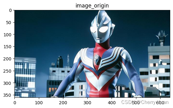
img = Image.open("TIGA.jpg")

plt.title("image_origin")
plt.imshow(img,cmap="brg")
plt.show()

#将图像数据转化成numpy类型的数组
img_arr = np.array(img)

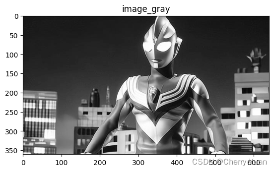
#将图像转化成灰度图
image = img_arr[:,:,0] * 0.299 + img_arr[:,:,1] * 0.587 + img_arr[:,:,2] * 0.114
image = np.ceil(image)   #对数组数据向上取整

plt.title("image_gray")
plt.imshow(image,cmap="gray")
plt.show()

height,width = image.shape


# #生成图像的直方图数据
hist = np.zeros((256,1))
for i in range(height):
    for j in range(width):
        hist[int(image[i,j]),0] += 1

        
#步骤二：全局阈值计算

#设置预定义值
delta_T = 1
        
#获取灰度级
grayscale = range(256)

#像素总数
num_pixels = height * width
        
#根据直方图数据计算灰度值的总和
total_gray = np.dot(hist[:,0],grayscale)

#计算整个图像的平均灰度值，以作为预设的灰度值阈值初值
T = round(total_gray / num_pixels)    #round()向下取整

#根据阈值处置生成两个集合（当然循环操作）
while True:
    num_G1 = np.sum(hist[:T,0])  #统计G1的像素数量
    sum_G1 = np.dot(hist[:T,0],range(T))   #统计G1的灰度值总和
    num_G2 = num_pixels - num_G1     #统计G2的像素数量
    sum_G2 = total_gray - sum_G1     #统计G2的灰度值总和
    
    #分别求两个集合的平均灰度(记得一定要取整)
    m1 = round(sum_G1 / num_G1)
    m2 = round(sum_G2 / num_G2)
    
    #计算新的阈值Tnew
    Tnew = round((m1 + m2) / 2)
    
    #查看循环过程中前后两次迭代得到的阈值之间的差值，是否小于预定一直delta_T（可以理解为收敛）
    if abs(T - Tnew) < delta_T:   #等价于T = Tnew
        break
    else:
        T = Tnew

print("全局最优阈值：" + str(T))

#全局阈值已经得到了，接下来开始设置阈值处理的内容

#步骤三：阈值处理

#创建阈值处理后的新图像
image_threshold = np.zeros((height,width))
for i in range(height):
    for j in range(width):
        if image[i,j] < T:
            image_threshold[i,j] = 0
        else:
            image_threshold[i,j] = 255

plt.title("image_threshold_total")
plt.imshow(image_threshold,cmap="gray")
plt.show()

请添加图片描述
在这里插入图片描述

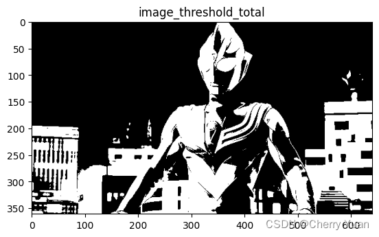
上述代码中出现的阈值初值为灰度图平均灰度，其实也可以换成别的初值，大家可以换成别的试一试。

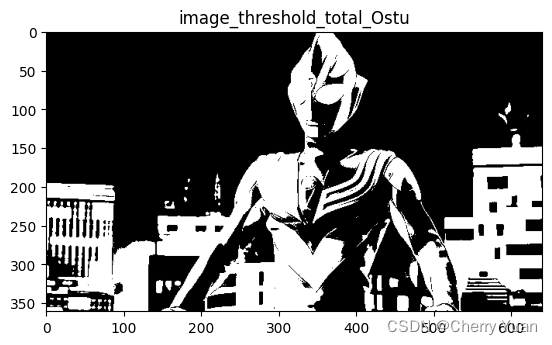
使用Otsu方法的最优全局阈值处理

该方法使用最大化类间方差，在全局阈值阈值处理的基础上考虑不同阈值区分开的两个集合各自像素数的占比、两个集合由此的类间方差，公式如下： $\sigma^2=P_1(m_1-m)^2+P_2(m_2-m)^2$
其中， $P_1$ 与 $P_2$ 分别表示由阈值分割成的两个集合各自的像素占比情况。 $m_1$ 与 $m_2$ 分别表示两个集合各自的平均灰度值， $m$ 表示整个图像的平均灰度值。
在得到类间方差的过程中，用以分割像素灰度的阈值变化范围是 $[0, L - 1]$ ， $L$ 表示图像灰度级。我们的实验所使用的是灰度级为256的图像，因此分割灰度的范围是 $[0, 255]$ ，且都是整数。
由此产生的256种类间方差，必然存在最大值，能使得类间方差最大的阈值 $T$ 就是我们需要的最优阈值。

import numpy as np
from PIL import Image
import matplotlib.pyplot as plt

#步骤一：获取图像的灰度直方图数据

#读取图像数据
img = Image.open("TIGA.jpg")

plt.title("image_origin")
plt.imshow(img,cmap="brg")
plt.show()

#将图像数据转化成numpy类型的数组
img_arr = np.array(img)

#将图像转化成灰度图
image = img_arr[:,:,0] * 0.299 + img_arr[:,:,1] * 0.587 + img_arr[:,:,2] * 0.114
image = np.ceil(image)   #对数组数据向上取整

plt.title("image_gray")
plt.imshow(image,cmap="gray")
plt.show()

height,width = image.shape


# #生成图像的直方图数据
hist = np.zeros((256,1))
for i in range(height):
    for j in range(width):
        hist[int(image[i,j]),0] += 1

        
#步骤二：类间方差计算
        
#获取灰度级
grayscale = range(256)

#像素总数
num_pixels = height * width
        
#根据直方图数据计算灰度值的总和
total_gray = np.dot(hist[:,0],grayscale)

#计算整个图像的平均灰度值，以作为预设的灰度值阈值初值
m = total_gray / num_pixels  

#创建存储类间方差的数组（两个集合一共是由256种不同的阈值分割的，因此产生的类间方差也就有256种）
sigma_array = np.zeros(256)

#根据阈值处置生成两个集合（当然循环操作）
for T in range(256):
    num_G1 = np.sum(hist[:T,0])  #统计G1的像素数量
    sum_G1 = np.dot(hist[:T,0],range(T))   #统计G1的灰度值总和
    num_G2 = num_pixels - num_G1     #统计G2的像素数量
    sum_G2 = total_gray - sum_G1     #统计G2的灰度值总和
    
    P1 = num_G1 / num_pixels
    P2 = num_G2 / num_pixels
    
    #分别求两个集合的平均灰度(记得一定要取整)
    m1 = (sum_G1 / num_G1) if  num_G1 > 0 else 0
    m2 = (sum_G2 / num_G2) if  num_G2 > 0 else 0
    
    #计算当前迭代所用阈值得到的类间方差
    sigma_array[T] = P1 * (m1 - m) ** 2  + P2 * (m2 - m) ** 2

#步骤三：根据上一步骤得到的类间方差数组，找寻最大类间方差对应的阈值，作为最优阈值。
max = np.max(sigma_array)
max_index = np.argmax(sigma_array)    # numpy.argmax()  Returns the indices of the maximum values along an axis.

T = max_index

print("使用的Otsu后的全局最优阈值：" + str(T))

#步骤四：阈值处理

#创建阈值处理后的新图像
image_threshold = np.zeros((height,width))
for i in range(height):
    for j in range(width):
        if image[i,j] < T:
            image_threshold[i,j] = 0
        else:
            image_threshold[i,j] = 255

plt.title("image_threshold_total_Ostu")
plt.imshow(image_threshold,cmap="gray")
plt.show()