


吴恩达Deep Learning编程作业 Course1-神经网络和深度学习-第三周作业
Building your Deep Neural Network: Step by Step 一步步建立你的深度神经网络
学习目标:
- 使用非线性激活函数,如Relu等,提升你的模型。
- 建立一个更深层的神经网络。
- 实现一个易于使用的神经网络类
注意符号的意思:
- 上标[ l l l]表示第 l t h l^{th} lth层。
-
- a [ L ] a^{[L]} a[L]是第 L [ t h ] L^{[th]} L[th]层的激活值。
- 上标(i)表示第 i t h i^{th} ith个样本
-
- 比如 x ( i ) x^{(i)} x(i)是第 i t h i^{th} ith个训练样本。
- 下标i表示第几个向量。
-
- a i [ l ] a^{[l]}_i ai[l]表示第 l t h l^{th} lth第 i t h i^{th} ith个向量。
1.需要引入的包
numpy:是Python用于科学计算的基本包。
matplotlib:python用于画图的库。
dnn_utils:一个工具包,为神经网络模型的搭建提供工具。
testCases:提供测试来评估我们的函数。
使用np.random.seed(1)是为了保证你得到的数据结果和我的一致,如果你有把握自己做的正确可以不使用它。
import numpy as np
import matplotlib.pyplot as plt
from Utils.testCases import *
from Utils.dnn_utils import sigmoid,sigmoid_backward,relu,relu_backward

#调整画布参数
plt.rcParams['figure.figsize'] = (5.0, 4.0)
plt.rcParams['image.interpolation'] = 'nearest'
plt.rcParams['image.cmap'] = 'gray'

np.random.seed(1)
2.本次需要完成的主要内容
1.为建立L层神经网络,初始化两层网络的参数。
2. 实现前向传播模块(如下图紫色部分所示)。
- 完成前向传播中的线性部分(得到 Z [ l ] Z^{[l]} Z[l])。
- 使用激活函数(relu/sigmoid)
- 将以上两步整合到一个新的函数中。
- 在第一层到第L-1层使用激活函数Relu,在最后一层使用Sigmoid函数。
3.计算损失
4.实现反向传播函数。
- 完成反向传播中线性部分。
- 利用激活函数的导数实现梯度下降。
- 将前面两步整合到一个函数中。
- 在第一层到第L-1层中使用激活函数Relu,在最后一层中使用Sigmid函数。
5.更新所有的参数。

3.初始化
我们将编写两个工具函数来实现我们的模型,这两个函数主要用来初始化参数。第一个函数用来初始化两层模型的参数,第二个将把这种初始化参数的过程推广到第L层。
3.1 两层神经网络
模型的结构:LINEAR -> RELU -> LINEAR -> SIGMOID.
对权重矩阵随机初始化。使用np.random.randn(shape)*0.01。
初始化偏差矩阵为0。
代码:
def initialize_parameters(n_x, n_h, n_y):
    """
    :param n_x: 输入特征个数
    :param n_h: 隐藏层个数
    :param n_y: 输出层个数
    :return:
    Returns:
        W1:--权重矩阵 (n_h, n_x)
        b1:--偏置矩阵 (n_h, 1)
        W2:--权重矩阵 (n_y, n_h)
        b2:--偏置矩阵 (n_y, 1)
    """
    np.random.seed(1)

    W1 = np.random.randn(n_h, n_x) * 0.01
    b1 = np.zeros(shape=(n_h, 1))
    W2 = np.random.randn(n_y, n_h) * 0.01
    b2 = np.zeros(shape=(n_y, 1))

    assert (W1.shape == (n_h, n_x))
    assert (b1.shape == (n_h, 1))
    assert (W2.shape == (n_y, n_h))
    assert (b2.shape == (n_y, 1))

    parameters = {"W1": W1,
                  "b1": b1,
                  "W2": W2,
                  "b2": b2}

    return parameters
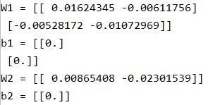
调用:
if __name__ == '__main__':
    parameters = initialize_parameters(2, 2, 1)
    print("W1 = " + str(parameters["W1"]))
    print("b1 = " + str(parameters["b1"]))
    print("W2 = " + str(parameters["W2"]))
    print("b2 = " + str(parameters["b2"]))
运行结果:
3.2 L层神经网络实现
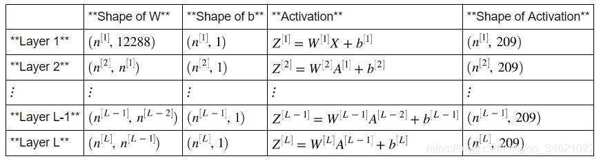
以输入X(12288, 209)为例,表中标出了每个参数的维度。
我们以矩阵为例计算:
W
=
[
j
k
l
m
n
o
p
q
r
]
X
=
[
a
b
c
d
e
f
g
h
i
]
b
=
[
s
t
u
]
W = \left[\begin{matrix} j & k & l \\m & n & o \\p & q & r \end{matrix} \right] X = \left[\begin{matrix} a & b & c \\d & e & f\\g & h & i\end{matrix} \right] b = \left[\begin{matrix} s\\ t\\ u\end{matrix} \right]
W=⎣⎡jmpknqlor⎦⎤X=⎣⎡adgbehcfi⎦⎤b=⎣⎡stu⎦⎤
W
X
+
b
=
[
(
j
a
+
k
d
+
l
g
)
+
s
(
j
b
+
k
e
+
l
h
)
+
s
(
j
c
+
k
f
+
l
i
)
+
s
(
m
a
+
n
d
+
o
g
)
+
t
(
m
b
+
n
e
+
o
h
)
+
t
(
m
c
+
n
f
+
o
i
)
+
t
(
p
a
+
q
d
+
r
g
)
+
u
(
p
b
+
q
e
+
r
h
)
+
u
(
p
c
+
q
f
+
r
i
)
+
u
]
WX + b = \left[\begin{matrix}(ja + kd + lg) + s & (jb + ke + lh) + s & (jc + kf + li) + s\\ (ma + nd + og) + t & (mb + ne + oh) + t & (mc + nf + oi) + t \\(pa + qd + rg) + u & (pb + qe + rh ) + u & (pc + qf + ri) + u\end{matrix} \right]
WX+b=⎣⎡(ja+kd+lg)+s(ma+nd+og)+t(pa+qd+rg)+u(jb+ke+lh)+s(mb+ne+oh)+t(pb+qe+rh)+u(jc+kf+li)+s(mc+nf+oi)+t(pc+qf+ri)+u⎦⎤
了解完矩阵的运算过程以后,接下来我们就一起初始化L层神经网络的参数。
注意:
在L-1层前我们使用的都是Relu激活函数,第L层使用的是Sigmoid激活函数。
初始化权重矩阵我们使用的是np.random.randn(shape) ×0.01。
代码:
def initialize_parameters_deep(layer_dims):
    np.random.seed(3)
    parameters = {}
    L = len(layer_dims)
    for l in range(1, L):
        parameters['W' + str(l)] = np.random.randn(layer_dims[l], layer_dims[l - 1]) * 0.01
        parameters['b' + str(l)] = np.zeros((layer_dims[l], 1))
        assert (parameters['W' + str(l)].shape == (layer_dims[l], layer_dims[l - 1]))
        assert (parameters['b' + str(l)].shape == (layer_dims[l], 1))

    return parameters
测试:
 	parameters = initialize_parameters_deep([5, 4, 3])
    print("W1 = " + str(parameters["W1"]))
    print("b1 = " + str(parameters["b1"]))
    print("W2 = " + str(parameters["W2"]))
    print("b2 = " + str(parameters["b2"]))
运行结果:

4.前向传播模型
4.1 线性向前
现在已经初始化了参数,接下来将执行正向传播模块。我们将首先实现一些基本功能,稍后在实现模型时将使用这些功能。我们将按如下顺序完成三个功能:
1.线性
2.线性->激活函数(Relu和Sigmoid)
3.[线性->Relu] × (L - 1)->线性->Sigmoid
线性向前模型主要[]计算下列等式。
Z
[
l
]
=
W
[
l
]
A
[
l
−
1
]
+
b
[
l
]
Z^{[l]} = W^{[l]}A^{[l-1]} + b^{[l]}
Z[l]=W[l]A[l−1]+b[l]
A
[
0
]
=
X
A^{[0]} = X
A[0]=X
代码实现:
def linear_forward(A, W, b):
    Z = np.dot(W, A) + b
    assert (Z.shape == (W.shape[0], A.shape[1]))
    cache = (A, W, b)

    return Z,cache
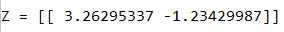
代码调用:
A, W, b = linear_forward_test_case()
    Z, linear_cache = linear_forward(A, W, b)
    print("Z = " + str(Z))
运行结果:
4.2 线性激活函数
在这里,我们主要使用两种激活函数:
1.
s
i
g
m
o
i
d
sigmoid
sigmoid:
σ
(
Z
)
=
σ
(
W
A
+
b
)
=
\sigma(Z) = \sigma(WA + b) =
σ(Z)=σ(WA+b)=
1
1
+
e
−
(
W
A
+
b
)
1 \over {1+e^{-(WA + b)}}
1+e−(WA+b)1
2.
R
e
l
u
Relu
Relu:
A
=
R
e
l
u
(
Z
)
=
m
a
x
(
0
,
Z
)
A = Relu(Z) = max(0,Z)
A=Relu(Z)=max(0,Z)
为了方便计算,我们将线性计算和激活函数合为一个式子,如下式所示:
A
[
l
]
=
g
(
Z
[
l
]
)
A^{[l]} = g(Z^{[l]})
A[l]=g(Z[l]) =
g
(
W
[
l
]
A
[
l
−
1
]
+
b
[
l
]
)
g(W^{[l]}A^{[l-1]} + b^{[l]})
g(W[l]A[l−1]+b[l]),其中函数g指的就是sigmoid或者Relu。
代码:
#前向传播中计算激活函数的值
def linear_activation_forward(A_prev, W, b, activation):
    """
    :param A_prev: 上一层的激活值
    :param W: 这一层的权重矩阵
    :param b: 这一层的偏置值
    :param activation:选择的激活函数名
    :return:
    """
    if activation == "sigmoid":
        Z, linear_cache = linear_forward(A_prev, W, b)
        A, activation_cache = sigmoid(Z) #activation_cache中包含反向传播要使用的A和Z
    elif activation == "relu":
        Z, linear_cache = linear_forward(A_prev, W, b)
        A, activation_cache = relu(Z)
    assert (A.shape == (W.shape[0], A_prev.shape[1]))
    cache = (linear_cache, activation_cache)
    return A, cache
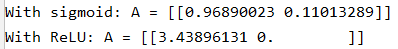
调用代码:
 A_prev, W, b = linear_activation_forward_test_case()
    A, linear_activation_cache = linear_activation_forward(A_prev, W, b, activation="sigmoid")
    print("With sigmoid: A = " + str(A))
    A, linear_activation_cache = linear_activation_forward(A_prev, W, b, activation="relu")
    print("With ReLU: A = " + str(A))
运行结果:
4.4 L层模型构建
下图是L层模型示例图:
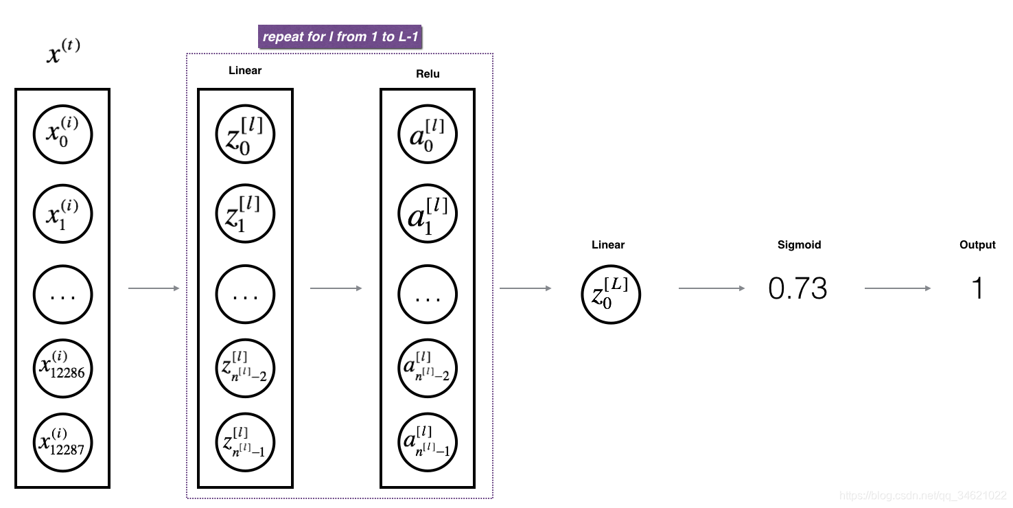
接下来我们就实现这个模型的前向传播:
代码:
def L_model_forward(X, parameters):
    caches = []
    A = X
    L = len(parameters)//2  #" / "就表示 浮点数除法,返回浮点结果;" // "表示整数除法。
    for i in range(1, L):
        A_prev = A
        A, cache = linear_activation_forward(A_prev, parameters['W' + str(1)], parameters['b' + str(1)], activation='relu')
        caches.append(cache)

    AL, cache = linear_activation_forward(A, parameters['W' + str(L)], parameters['b' + str(L)], activation='sigmoid')

    caches.append(cache)
    assert(AL.shape == (1, X.shape[1]))

    return AL, caches
调用:
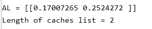
    X, parameters = L_model_forward_test_case()
    AL, caches = L_model_forward(X, parameters)
    print("AL = " + str(AL))
    print("Length of caches list = " + str(len(caches)))
运行结果:
5. 代价函数
数学公式如下:
J
=
−
1
m
∑
i
=
1
m
(
y
(
i
)
log
(
a
[
L
]
(
i
)
)
+
(
1
−
y
(
i
)
)
log
(
1
−
a
[
L
]
(
i
)
)
)
J = -\frac{1}{m} \sum\limits_{i = 1}^{m} (y^{(i)}\log\left(a^{[L] (i)}\right) + (1-y^{(i)})\log\left(1- a^{[L](i)}\right))
J=−m1i=1∑m(y(i)log(a[L](i))+(1−y(i))log(1−a[L](i)))
代码:
def compute_cost(AL, Y):
    m = Y.shape[1]
    cost = (-1 / m) * np.sum(np.multiply(Y, np.log(AL)) + np.multiply(1 - Y, np.log(1 - AL)))
    cost = np.squeeze(cost)
    assert(cost.shape == ())
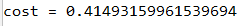
调用:
    Y, AL = compute_cost_test_case()
    print("cost = " + str(compute_cost(AL, Y)))
运行结果:
6. 反向传播模型
计算模型:

6.1 反向线性
对于
l
l
l层,最后的线性计算公式为:
Z
[
l
]
=
W
[
l
]
A
[
l
−
1
]
+
b
[
l
]
Z^{[l]} = W^{[l]}A^{[l - 1]} + b^{[l]}
Z[l]=W[l]A[l−1]+b[l].
假设我们已经计算得到了:
d
Z
[
l
]
=
dZ^{[l]} =
dZ[l]=
α
L
α
Z
[
l
]
\alpha L \over \alpha Z^{[l]}
αZ[l]αL,那么我们还需要得到
(
d
W
[
l
]
,
d
b
[
l
]
,
d
A
[
l
−
1
]
)
(dW^{[l]},db^{[l]},dA^{[l - 1]})
(dW[l],db[l],dA[l−1])
具体计算形式如下图所示:
数学公式推导:
d
W
[
l
]
=
dW^{[l]} =
dW[l]=
α
L
α
W
[
l
]
=
{\alpha L \over \alpha W^{[l]} }=
αW[l]αL=
1
m
d
Z
[
l
]
A
[
l
−
1
]
T
{1 \over m} dZ^{[l]}A^{[l-1]T}
m1dZ[l]A[l−1]T
d b [ l ] = db^{[l]} = db[l]= α L α b [ l ] = {\alpha L \over \alpha b^{[l]}} = αb[l]αL= 1 m ∑ i = 1 m d Z [ l ] ( i ) {1 \over m}\sum_{i=1}^m{dZ^{[l](i)}} m1∑i=1mdZ[l](i)
d A [ l − 1 ] = dA^{[l - 1]} = dA[l−1]= α L α A [ l − 1 ] = {\alpha L \over \alpha A^{[l-1]} }= αA[l−1]αL= W [ l ] T d Z [ l ] W^{[l]T}dZ^{[l]} W[l]TdZ[l]
代码如下:
def linear_backward(dZ, cache):
    A_prev, W, b = cache
    m = A_prev.shape[1]
    dW = np.dot(dZ, A_prev.T)/m
    db = np.sum(dZ, axis=1, keepdims=True) / m
    dA_prev = np.dot(cache[1].T, dZ)
    assert (dA_prev.shape == A_prev.shape)
    assert (dW.shape == W.shape)
    assert (isinstance(db, float))

    return dA_prev, dW, db
调用:
dZ, linear_cache = linear_backward_test_case()
dA_prev, dW, db = linear_backward(dZ, linear_cache)
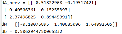
print("dA_prev = " + str(dA_prev))
print("dW = " + str(dW))
print("db = " + str(db))
运行结果:
6.2 反向线性激活计算
在上一步中我们计算了线性球道的部分,但是我们在计算过程中还使用了非线性激活函数,因此在这一步中我们也要计算非线性激活函数的导数。
在前向传播中我们使用了两个非线性激活函数:Relu和sigmoid。
1.sigmoid的导数:
g
′
(
Z
)
=
g
(
Z
)
(
1
−
g
(
Z
)
)
g^{'}(Z) = g(Z)(1-g(Z))
g′(Z)=g(Z)(1−g(Z))
2.relu的导数:
g
′
(
Z
)
=
{
0.01
Z
,
i
f
z
<
0
1
,
i
f
z
>
0
u
n
d
e
f
i
n
e
d
,
i
f
z
=
0
g^{'}(Z) = \begin{cases} 0.01Z, &if\ z<0\\ 1,&if\ z>0\\ undefined ,&if\ z= 0 \end{cases}
g′(Z)=⎩⎪⎨⎪⎧0.01Z,1,undefined,if z<0if z>0if z=0
d
Z
[
l
]
=
d
A
[
l
]
∗
g
′
(
Z
[
l
]
)
dZ^{[l]} = dA^{[l]} * g^{'}(Z^{[l]})
dZ[l]=dA[l]∗g′(Z[l])
代码:
def linear_activation_backward(dA, cache, activation):
    """
    :param dA: L层的激活值
    :param cache: linear_cache线性参数A[L-1],W,b;activation_cache第L层激活值A
    :param activation:激活函数的名字
    :return:
    """
    linear_cache, activation_cache = cache
    if activation == 'sigmoid':
        dZ = sigmoid_backward(dA, activation_cache)

    elif activation == 'relu':
        dZ = relu_backward(dA, activation_cache)
    dA_prev, dW, db = linear_backward(dZ, linear_cache)

    return dA_prev, dW, db
调用:
AL, linear_activation_cache = linear_activation_backward_test_case()
    dA_prev, dW, db = linear_activation_backward(AL, linear_activation_cache, activation="sigmoid")
    print("sigmoid:")
    print("dA_prev = " + str(dA_prev))
    print("dW = " + str(dW))
    print("db = " + str(db) + "\n")

    dA_prev, dW, db = linear_activation_backward(AL, linear_activation_cache, activation="relu")
    print("relu:")
    print("dA_prev = " + str(dA_prev))
    print("dW = " + str(dW))
    print("db = " + str(db))
结果:

6.3 L层模型的反向传播
计算模型图如下:

在下面的计算中我们需要计算
d
A
L
=
α
L
α
A
[
L
]
dAL = {\alpha L \over \alpha A^{[L]}}
dAL=αA[L]αL,因为
L
(
a
,
y
)
=
−
(
y
log
(
a
)
+
(
1
−
y
)
log
(
1
−
a
)
)
L(a, y) = -(y\log (a) + (1 - y)\log (1 - a))
L(a,y)=−(ylog(a)+(1−y)log(1−a))
对上式求导得:
α
L
α
a
=
−
(
y
a
−
(
1
−
y
)
(
1
−
a
)
)
{\alpha L \over \alpha a} = -({y \over a} - {(1 - y) \over (1 - a)})
αaαL=−(ay−(1−a)(1−y))
因此我们要用到的主要代码:
dAL = - (np.divide(Y, AL) - np.divide(1 - Y, 1 - AL))
代码:
def L_model_backward(AL, Y, caches):
    """
    :param AL: 前向传播中计算出的第L层得激活值,来自L_model_forward()
    :param Y: 正确的分类标签
    :param caches: 用来存储每层的激活值,0~L-2层的Relu函数激活值,第L-1层的sigmoid函数激活值(A,Z)
    :return: 每一层的dA,dW,db
    """
    grads = {}
    L = len(caches) #计算出一共有多少层
    Y = Y.reshape(AL.shape) #重新定义Y的维数,方便后续计算

    dAL = -(np.divide(Y, AL) - np.divide(1 - Y, 1 - AL))
    current_cache = caches[-1] #A 、cache={linear_cache、activation_cache}
    grads["dA" + str(L)], grads["dW" + str(L)], grads["db" + str(L)] = linear_activation_backward(dAL, current_cache, "sigmoid")

    for l in reversed(range(L - 1)):#不包含L-1
        current_cache = caches[l]
        grads["dA" + str(l + 1)], grads["dW" + str(l + 1)], grads["db" + str(l + 1)] = linear_activation_backward(grads["dA" + str(l + 2)], current_cache, "relu")
    return grads
调用:
AL, Y_assess, caches = L_model_backward_test_case()
grads = L_model_backward(AL, Y_assess, caches)
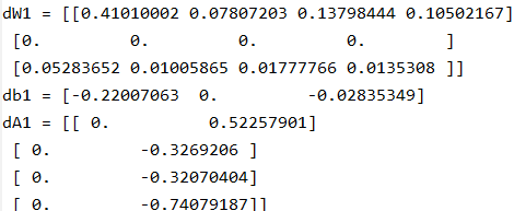
print("dW1 = " + str(grads["dW1"]))
print("db1 = " + str(grads["db1"]))
print("dA1 = " + str(grads["dA1"]))
运行结果:
6.5 更新参数
使用数学公式:
b
[
l
]
=
b
[
l
]
−
a
d
b
[
l
]
b^{[l]} = b^{[l]} - adb^{[l]}
b[l]=b[l]−adb[l],其中a是学习率。
代码:
def update_parameters(parameters, grads, learning_rate):
    """
    :param parameters: 包含参数的字典
    :param grads: 梯度值
    :param learning_rate:学习率
    :return:
    """
    L = len(parameters) // 2
    for l in range(L):
        parameters["W" + str(l + 1)] = parameters["W" + str(l + 1)] - learning_rate * grads["dW" + str(l + 1)]
        parameters["b" + str(l + 1)] = parameters["b" + str(l + 1)] - learning_rate * grads["db" + str(l + 1)]

    return parameters
调用:
parameters, grads = update_parameters_test_case()
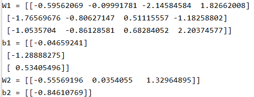
parameters = update_parameters(parameters, grads, 0.1)
print("W1 = " + str(parameters["W1"]))
print("b1 = " + str(parameters["b1"]))
print("W2 = " + str(parameters["W2"]))
print("b2 = " + str(parameters["b2"]))
运行结果:
接下来我们使用自己的这些模型来搭建一个两层的神经网络。
请看下一篇文章。
下面是本次代码用到的库代码:
库代码
dnn_utils.py
# dnn_utils.py
import numpy as np

def sigmoid(Z):
    """
    Implements the sigmoid activation in numpy

    Arguments:
    Z -- numpy array of any shape

    Returns:
    A -- output of sigmoid(z), same shape as Z
    cache -- returns Z as well, useful during backpropagation
    """

    A = 1/(1+np.exp(-Z))
    cache = Z

    return A, cache

def sigmoid_backward(dA, cache):
    """
    Implement the backward propagation for a single SIGMOID unit.

    Arguments:
    dA -- post-activation gradient, of any shape
    cache -- 'Z' where we store for computing backward propagation efficiently

    Returns:
    dZ -- Gradient of the cost with respect to Z
    """

    Z = cache

    s = 1/(1+np.exp(-Z))
    dZ = dA * s * (1-s)

    assert (dZ.shape == Z.shape)

    return dZ

def relu(Z):
    """
    Implement the RELU function.

    Arguments:
    Z -- Output of the linear layer, of any shape

    Returns:
    A -- Post-activation parameter, of the same shape as Z
    cache -- a python dictionary containing "A" ; stored for computing the backward pass efficiently
    """

    A = np.maximum(0,Z)

    assert(A.shape == Z.shape)

    cache = Z
    return A, cache

def relu_backward(dA, cache):
    """
    Implement the backward propagation for a single RELU unit.

    Arguments:
    dA -- post-activation gradient, of any shape
    cache -- 'Z' where we store for computing backward propagation efficiently

    Returns:
    dZ -- Gradient of the cost with respect to Z
    """

    Z = cache
    dZ = np.array(dA, copy=True) # just converting dz to a correct object.

    # When z <= 0, you should set dz to 0 as well.
    dZ[Z <= 0] = 0

    assert (dZ.shape == Z.shape)

    return dZ
testCases_DNN.py
# testCase.py
import numpy as np


def linear_forward_test_case():
    np.random.seed(1)
    A = np.random.randn(3, 2)
    W = np.random.randn(1, 3)
    b = np.random.randn(1, 1)

    return A, W, b


def linear_activation_forward_test_case():
    np.random.seed(2)
    A_prev = np.random.randn(3, 2)
    W = np.random.randn(1, 3)
    b = np.random.randn(1, 1)
    return A_prev, W, b


def L_model_forward_test_case():
    np.random.seed(1)
    X = np.random.randn(4, 2)
    W1 = np.random.randn(3, 4)
    b1 = np.random.randn(3, 1)
    W2 = np.random.randn(1, 3)
    b2 = np.random.randn(1, 1)
    parameters = {"W1": W1,
                  "b1": b1,
                  "W2": W2,
                  "b2": b2}

    return X, parameters


def compute_cost_test_case():
    Y = np.asarray([[1, 1, 1]])
    aL = np.array([[.8, .9, 0.4]])

    return Y, aL


def linear_backward_test_case():
    np.random.seed(1)
    dZ = np.random.randn(1, 2)
    A = np.random.randn(3, 2)
    W = np.random.randn(1, 3)
    b = np.random.randn(1, 1)
    linear_cache = (A, W, b)
    return dZ, linear_cache


def linear_activation_backward_test_case():
    np.random.seed(2)
    dA = np.random.randn(1, 2)
    A = np.random.randn(3, 2)
    W = np.random.randn(1, 3)
    b = np.random.randn(1, 1)
    Z = np.random.randn(1, 2)
    linear_cache = (A, W, b)
    activation_cache = Z
    linear_activation_cache = (linear_cache, activation_cache)

    return dA, linear_activation_cache


def L_model_backward_test_case():
    np.random.seed(3)
    AL = np.random.randn(1, 2)
    Y = np.array([[1, 0]])

    A1 = np.random.randn(4, 2)
    W1 = np.random.randn(3, 4)
    b1 = np.random.randn(3, 1)
    Z1 = np.random.randn(3, 2)
    linear_cache_activation_1 = ((A1, W1, b1), Z1)

    A2 = np.random.randn(3, 2)
    W2 = np.random.randn(1, 3)
    b2 = np.random.randn(1, 1)
    Z2 = np.random.randn(1, 2)
    linear_cache_activation_2 = ((A2, W2, b2), Z2)

    caches = (linear_cache_activation_1, linear_cache_activation_2)

    return AL, Y, caches


def update_parameters_test_case():
    np.random.seed(2)
    W1 = np.random.randn(3, 4)
    b1 = np.random.randn(3, 1)
    W2 = np.random.randn(1, 3)
    b2 = np.random.randn(1, 1)
    parameters = {"W1": W1,
                  "b1": b1,
                  "W2": W2,
                  "b2": b2}
    np.random.seed(3)
    dW1 = np.random.randn(3, 4)
    db1 = np.random.randn(3, 1)
    dW2 = np.random.randn(1, 3)
    db2 = np.random.randn(1, 1)
    grads = {"dW1": dW1,
             "db1": db1,
             "dW2": dW2,
             "db2": db2}

    return parameters, grads


 629
629


 被折叠的 条评论
为什么被折叠?
被折叠的 条评论
为什么被折叠?
 到【灌水乐园】发言


