【深度学习-吴恩达】L1-4 深层神经网络作业

最新推荐文章于 2023-08-29 09:23:42 发布

JackSerin

最新推荐文章于 2023-08-29 09:23:42 发布

阅读量644

点赞数

分类专栏：深度学习文章标签：深度学习神经网络 python

本文链接：https://blog.csdn.net/u011315681/article/details/126043874

版权

深度学习专栏收录该内容

14 篇文章 2 订阅

订阅专栏

L1 深度学习概论

4 深层神经网络

作业链接：吴恩达《深度学习》 - Heywhale.com

0 作业任务

构建一个任意层数的深度神经网络

实现构建深度神经网络所需的所有函数
使用这些函数构建一个用于图像分类的深度神经网络

学习目标：

使用ReLU等非线性单元改善模型
建立更深的神经网络
实现一个易于使用的神经网络类

1 深度神经网络的函数

1.1 导入安装包

numpy是Python科学计算的基本包
matplotlib是在Python中常用的绘制图形的库
dnn_utils为此笔记本提供了一些必要的函数
testCases提供了一些测试用例来评估函数的正确性
np.random.seed（1）使所有随机函数调用保持一致

import time
import numpy as np
import h5py
import matplotlib.pyplot as plt
import scipy
from PIL import Image
from scipy import ndimage
from testCases_v2 import *
from dnn_utils_v2 import *

%matplotlib inline
plt.rcParams['figure.figsize'] = (5.0, 4.0) # set default size of plots
plt.rcParams['image.interpolation'] = 'nearest'
plt.rcParams['image.cmap'] = 'gray'

%load_ext autoreload
%autoreload 2

np.random.seed(1)

1.2 大纲

实现如下函数：

初始化两层的网络和L层的神经网络参数
实现正向传播模块
- 完成正向传播
- 提供激活函数
- 将前两个步骤合并为前向函数
- 堆叠前向函数，并在末尾添加sigmoid，合成L_model_forward函数
计算损失
实现反向传播模块
- 完成反向传播
- 提供激活函数的梯度
- 将前两个步骤组合成反向函数
- 堆叠反向函数，并在新的L_model_backward函数中后向添加sigmoid函数
最后更新参数

实现过程图解如下所示：

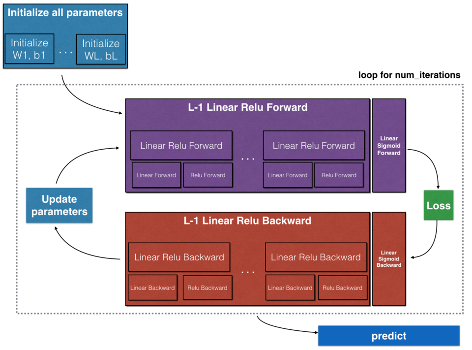
Tips：

对于每个正向函数，都有一个对应的反向函数
- 正向传播模块缓存一些数值

1.3 初始化

首先编写2个函数用来初始化模型的参数

第一个用于初始化两层模型的数据
第二个把初始化过程推广到L层模型上

1.3.1 2层神经网络

练习：创建并初始化2层神经网络的参数

# GRADED FUNCTION: initialize_parameters

def initialize_parameters(n_x, n_h, n_y):
    """
    Argument:
    n_x -- size of the input layer
    n_h -- size of the hidden layer
    n_y -- size of the output layer
    
    Returns:
    parameters -- python dictionary containing your parameters:
                    W1 -- weight matrix of shape (n_h, n_x)
                    b1 -- bias vector of shape (n_h, 1)
                    W2 -- weight matrix of shape (n_y, n_h)
                    b2 -- bias vector of shape (n_y, 1)
    """
    np.random.seed(1)
    
    W1 = np.random.randn(n_h, n_x)*0.01
    b1 = np.zeros((n_h,1))
    W2 = np.random.randn(n_y, n_h)*0.01
    b2 = np.zeros((n_y,1))
    
    assert(W1.shape == (n_h, n_x))
    assert(b1.shape == (n_h, 1))
    assert(W2.shape == (n_y, n_h))
    assert(b2.shape == (n_y, 1))
    
    parameters = {"W1": W1,
                  "b1": b1,
                  "W2": W2,
                  "b2": b2}
    
    return parameters

1.3.2 L层神经网络

练习：实现L层神经网络的初始化

def initialize_parameters_deep(layer_dims):
    """
    Arguments:
    layer_dims -- python array (list) containing the dimensions of each layer in our network
    
    Returns:
    parameters -- python dictionary containing your parameters "W1", "b1", ..., "WL", "bL":
                    Wl -- weight matrix of shape (layer_dims[l], layer_dims[l-1])
                    bl -- bias vector of shape (layer_dims[l], 1)
    """
    
    np.random.seed(3)
    parameters = {}
    L = len(layer_dims)  # number of layers in the network

    for l in range(1, L):
        parameters['W' + str(l)] = np.random.randn(layer_dims[l],layer_dims[l-1])*0.01
        parameters['b' + str(l)] = np.zeros((layer_dims[l],1))
        
        assert(parameters['W' + str(l)].shape == (layer_dims[l], layer_dims[l-1]))
        assert(parameters['b' + str(l)].shape == (layer_dims[l], 1))

        
    return parameters

1.4 正向传播模块

1.4.1 线性正向

练习：建立正向传播的线性部分

# GRADED FUNCTION: linear_forward
def linear_forward(A, W, b):
    """
    Implement the linear part of a layer's forward propagation.

    Arguments:
    A -- activations from previous layer (or input data): (size of previous layer, number of examples)
    W -- weights matrix: numpy array of shape (size of current layer, size of previous layer)
    b -- bias vector, numpy array of shape (size of the current layer, 1)

    Returns:
    Z -- the input of the activation function, also called pre-activation parameter 
    cache -- a python dictionary containing "A", "W" and "b" ; stored for computing the backward pass efficiently
    """
    
    Z = np.dot(W,A) + b
    
    assert(Z.shape == (W.shape[0], A.shape[1]))
    cache = (A, W, b)
    
    return Z, cache

1.4.2 正向线性激活函数

练习：实现 LINEAR->ACTIVATION 层的正向传播

def linear_activation_forward(A_prev, W, b, activation):
    """
    Implement the forward propagation for the LINEAR->ACTIVATION layer

    Arguments:
    A_prev -- activations from previous layer (or input data): (size of previous layer, number of examples)
    W -- weights matrix: numpy array of shape (size of current layer, size of previous layer)
    b -- bias vector, numpy array of shape (size of the current layer, 1)
    activation -- the activation to be used in this layer, stored as a text string: "sigmoid" or "relu"

    Returns:
    A -- the output of the activation function, also called the post-activation value 
    cache -- a python dictionary containing "linear_cache" and "activation_cache";
             stored for computing the backward pass efficiently
    """
    
    if activation == "sigmoid":
        # Inputs: "A_prev, W, b". Outputs: "A, activation_cache".
        Z, linear_cache = linear_forward(A_prev,W,b)
        A, activation_cache = sigmoid(Z)
    
    elif activation == "relu":
        # Inputs: "A_prev, W, b". Outputs: "A, activation_cache".
        Z, linear_cache = linear_forward(A_prev,W,b)
        A, activation_cache = relu(Z)
    
    assert (A.shape == (W.shape[0], A_prev.shape[1]))
    cache = (linear_cache, activation_cache)

    return A, cache

1.4.3 L层模型

练习：实现L层模型的正向传播

# GRADED FUNCTION: L_model_forward
def L_model_forward(X, parameters):
    """
    Implement forward propagation for the [LINEAR->RELU]*(L-1)->LINEAR->SIGMOID computation
    
    Arguments:
    X -- data, numpy array of shape (input size, number of examples)
    parameters -- output of initialize_parameters_deep()
    
    Returns:
    AL -- last post-activation value
    caches -- list of caches containing:
                every cache of linear_relu_forward() (there are L-1 of them, indexed from 0 to L-2)
                the cache of linear_sigmoid_forward() (there is one, indexed L-1)
    """

    caches = []
    A = X
    # Ws and bs are in parameters
    # So the  below row calculates the number of layers in the neural network
    L = len(parameters) // 2 
    
    # Implement [LINEAR -> RELU]*(L-1). Add "cache" to the "caches" list.
    for l in range(1, L):
        A_prev = A 
        A, cache = linear_activation_forward(A_prev,parameters['W' + str(l)],parameters['b' + str(l)],activation = "relu")
        caches.append(cache)
    
    # Implement LINEAR -> SIGMOID. Add "cache" to the "caches" list.
    AL, cache = linear_activation_forward(A,parameters['W' + str(L)],parameters['b' + str(L)],activation = "sigmoid")
    caches.append(cache)
    
    assert(AL.shape == (1,X.shape[1]))
            
    return AL, caches

1.5 损失函数

练习：使用以下公式计算交叉熵损失 $J$ ：
$J=-\frac 1m\sum _{i=1}^m(y^{(i)}log(a^{[L](i)})+(1-y^{(i)})log(1-a^{[L](i)}))$

# GRADED FUNCTION: compute_cost
def compute_cost(AL, Y):
    """
    Implement the cost function defined by equation (7).

    Arguments:
    AL -- probability vector corresponding to your label predictions, shape (1, number of examples)
    Y -- true "label" vector (for example: containing 0 if non-cat, 1 if cat), shape (1, number of examples)

    Returns:
    cost -- cross-entropy cost
    """
    
    m = Y.shape[1]

    # Compute loss from aL and y.
    cost = -1 / m * np.sum(Y * np.log(AL) + (1-Y) * np.log(1-AL),axis=1,keepdims=True)
    
    # To make sure your cost's shape is what we expect (e.g. this turns [[17]] into 17).
    cost = np.squeeze(cost)      
    assert(cost.shape == ())
    
    return cost

1.6 反向传播模块

1.6.1 线性反向模块

练习：实现linear_backward（）

# GRADED FUNCTION: linear_backward
def linear_backward(dZ, cache):
    """
    Implement the linear portion of backward propagation for a single layer (layer l)

    Arguments:
    dZ -- Gradient of the cost with respect to the linear output (of current layer l)
    cache -- tuple of values (A_prev, W, b) coming from the forward propagation in the current layer

    Returns:
    dA_prev -- Gradient of the cost with respect to the activation (of the previous layer l-1), same shape as A_prev
    dW -- Gradient of the cost with respect to W (current layer l), same shape as W
    db -- Gradient of the cost with respect to b (current layer l), same shape as b
    """
    A_prev, W, b = cache
    m = A_prev.shape[1]

    dW = 1 / m * np.dot(dZ ,A_prev.T)
    db = 1 / m * np.sum(dZ,axis = 1 ,keepdims=True)
    dA_prev = np.dot(W.T,dZ) 

    
    assert (dA_prev.shape == A_prev.shape)
    assert (dW.shape == W.shape)
    assert (db.shape == b.shape)
    
    return dA_prev, dW, db

1.6.2 反向线性激活

练习：实现LINEAR->ACTIVATION层的反向传播

# GRADED FUNCTION: linear_activation_backward
def linear_activation_backward(dA, cache, activation):
    """
    Implement the backward propagation for the LINEAR->ACTIVATION layer.
    
    Arguments:
    dA -- post-activation gradient for current layer l 
    cache -- tuple of values (linear_cache, activation_cache) we store for computing backward propagation efficiently
    activation -- the activation to be used in this layer, stored as a text string: "sigmoid" or "relu"
    
    Returns:
    dA_prev -- Gradient of the cost with respect to the activation (of the previous layer l-1), same shape as A_prev
    dW -- Gradient of the cost with respect to W (current layer l), same shape as W
    db -- Gradient of the cost with respect to b (current layer l), same shape as b
    """
    linear_cache, activation_cache = cache
    
    if activation == "relu":
        dZ = relu_backward(dA, activation_cache)
        dA_prev, dW, db = linear_backward(dZ, linear_cache)
        
    elif activation == "sigmoid":
        dZ = sigmoid_backward(dA, activation_cache)
        dA_prev, dW, db = linear_backward(dZ, linear_cache)
    
    return dA_prev, dW, db

1.6.2 反向L层模型

练习：实现 [LINEAR->RELU] × (L-1) -> LINEAR -> SIGMOID 模型的反向传播

# GRADED FUNCTION: L_model_backward
def L_model_backward(AL, Y, caches):
    """
    Implement the backward propagation for the [LINEAR->RELU] * (L-1) -> LINEAR -> SIGMOID group
    
    Arguments:
    AL -- probability vector, output of the forward propagation (L_model_forward())
    Y -- true "label" vector (containing 0 if non-cat, 1 if cat)
    caches -- list of caches containing:
                every cache of linear_activation_forward() with "relu" (it's caches[l], for l in range(L-1) i.e l = 0...L-2)
                the cache of linear_activation_forward() with "sigmoid" (it's caches[L-1])
    
    Returns:
    grads -- A dictionary with the gradients
             grads["dA" + str(l)] = ...
             grads["dW" + str(l)] = ...
             grads["db" + str(l)] = ...
    """
    grads = {}
    L = len(caches) # the number of layers
    m = AL.shape[1]
    Y = Y.reshape(AL.shape) # after this line, Y is the same shape as AL

    # Initializing the backpropagation
    dAL = - (np.divide(Y, AL) - np.divide(1 - Y, 1 - AL))

    
    # Lth layer (SIGMOID -> LINEAR) gradients. Inputs: "AL, Y, caches". Outputs: "grads["dAL"], grads["dWL"], grads["dbL"]

    current_cache = caches[L-1]
    grads["dA" + str(L)], grads["dW" + str(L)], grads["db" + str(L)] = linear_activation_backward(dAL, current_cache, activation = "sigmoid")

      
    for l in reversed(range(L - 1)):
        # lth layer: (RELU -> LINEAR) gradients.
        # Inputs: "grads["dA" + str(l + 2)], caches". Outputs: "grads["dA" + str(l + 1)] , grads["dW" + str(l + 1)] , grads["db" + str(l + 1)] 

        current_cache = caches[l]
        dA_prev_temp, dW_temp, db_temp = linear_activation_backward(grads["dA" + str(l+2)], current_cache, activation = "relu")
        grads["dA" + str(l + 1)] = dA_prev_temp
        grads["dW" + str(l + 1)] = dW_temp
        grads["db" + str(l + 1)] = db_temp

    return grads

1.6.4 更新参数

练习：实现update_parameters（）以使用梯度下降来更新模型参数

# GRADED FUNCTION: update_parameters
def update_parameters(parameters, grads, learning_rate):
    """
    Update parameters using gradient descent
    
    Arguments:
    parameters -- python dictionary containing your parameters 
    grads -- python dictionary containing your gradients, output of L_model_backward
    
    Returns:
    parameters -- python dictionary containing your updated parameters 
                  parameters["W" + str(l)] = ... 
                  parameters["b" + str(l)] = ...
    """
    
    L = len(parameters) // 2 # number of layers in the neural network

    # Update rule for each parameter. Use a for loop.
    for l in range(L):
        parameters["W" + str(l+1)] =  parameters["W" + str(l+1)] - learning_rate * grads["dW" + str(l + 1)]
        parameters["b" + str(l+1)] = parameters["b" + str(l+1)] - learning_rate * grads["db" + str(l + 1)]
        
    return parameters

2 深度神经网络应用—图像分类

这一章使用的内容与上一章节联系紧密，相同操作不再赘述

2.1 数据集

这个数据集在L1-2作业中同样使用过，为 cats vs non-cats数据集

导入数据集并输出数据集相关参数

train_x_orig, train_y, test_x_orig, test_y, classes = load_data()

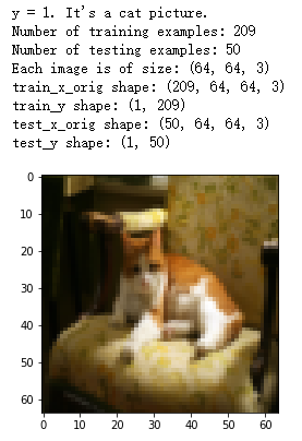
# Example of a picture
index = 7
plt.imshow(train_x_orig[index])
print ("y = " + str(train_y[0,index]) + ". It's a " + classes[train_y[0,index]].decode("utf-8") +  " picture.")

# Explore your dataset 
m_train = train_x_orig.shape[0]
num_px = train_x_orig.shape[1]
m_test = test_x_orig.shape[0]

print ("Number of training examples: " + str(m_train))
print ("Number of testing examples: " + str(m_test))
print ("Each image is of size: (" + str(num_px) + ", " + str(num_px) + ", 3)")
print ("train_x_orig shape: " + str(train_x_orig.shape))
print ("train_y shape: " + str(train_y.shape))
print ("test_x_orig shape: " + str(test_x_orig.shape))
print ("test_y shape: " + str(test_y.shape))

运行结果如下所示：

将图像转换为向量

# Reshape the training and test examples 
train_x_flatten = train_x_orig.reshape(train_x_orig.shape[0], -1).T   # The "-1" makes reshape flatten the remaining dimensions
test_x_flatten = test_x_orig.reshape(test_x_orig.shape[0], -1).T

# Standardize data to have feature values between 0 and 1.
train_x = train_x_flatten/255.
test_x = test_x_flatten/255.

print ("train_x's shape: " + str(train_x.shape))
print ("test_x's shape: " + str(test_x.shape))

2.2 2层神经网络

网络结构如下图所示：

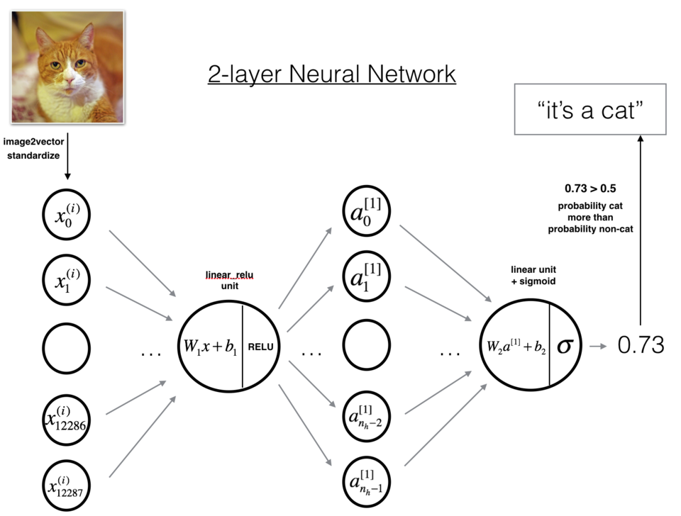
该模型可以总结为：INPUT -> LINEAR -> RELU -> LINEAR -> SIGMOID -> OUTPUT

练习：使用你在上一个作业中实现的辅助函数来构建具有以下结构的2层神经网络：LINEAR -> RELU -> LINEAR -> SIGMOID

### CONSTANTS DEFINING THE MODEL ####
n_x = 12288     # num_px * num_px * 3
n_h = 7
n_y = 1
layers_dims = (n_x, n_h, n_y)

# GRADED FUNCTION: two_layer_model
def two_layer_model(X, Y, layers_dims, learning_rate = 0.0075, num_iterations = 3000, print_cost=False):
    """
    Implements a two-layer neural network: LINEAR->RELU->LINEAR->SIGMOID.
    
    Arguments:
    X -- input data, of shape (n_x, number of examples)
    Y -- true "label" vector (containing 0 if cat, 1 if non-cat), of shape (1, number of examples)
    layers_dims -- dimensions of the layers (n_x, n_h, n_y)
    num_iterations -- number of iterations of the optimization loop
    learning_rate -- learning rate of the gradient descent update rule
    print_cost -- If set to True, this will print the cost every 100 iterations 
    
    Returns:
    parameters -- a dictionary containing W1, W2, b1, and b2
    """
    
    np.random.seed(1)
    grads = {}
    costs = [] # to keep track of the cost
    m = X.shape[1]  # number of examples
    (n_x, n_h, n_y) = layers_dims
    
    # Initialize parameters dictionary, by calling one of the functions you'd previously implemented
    parameters = initialize_parameters(n_x, n_h, n_y)
    
    # Get W1, b1, W2 and b2 from the dictionary parameters.
    W1 = parameters["W1"]
    b1 = parameters["b1"]
    W2 = parameters["W2"]
    b2 = parameters["b2"]
    
    # Loop (gradient descent)
    for i in range(0, num_iterations):
        # Forward propagation: LINEAR -> RELU -> LINEAR -> SIGMOID. Inputs: "X, W1, b1". Output: "A1, cache1, A2, cache2".
        A1, cache1 =linear_activation_forward(X, W1, b1, activation = "relu")
        A2, cache2 = linear_activation_forward(A1, W2, b2, activation = "sigmoid")
        
        # Compute cost
        cost = compute_cost(A2, Y)
        
        # Initializing backward propagation
        dA2 = - (np.divide(Y, A2) - np.divide(1 - Y, 1 - A2))
        
        # Backward propagation. Inputs: "dA2, cache2, cache1". Outputs: "dA1, dW2, db2; also dA0 (not used), dW1, db1".
        dA1, dW2, db2 = linear_activation_backward(dA2, cache2, activation = "sigmoid")
        dA0, dW1, db1 = linear_activation_backward(dA1, cache1, activation = "relu")
        
        # Set grads['dWl'] to dW1, grads['db1'] to db1, grads['dW2'] to dW2, grads['db2'] to db2
        grads['dW1'] = dW1
        grads['db1'] = db1
        grads['dW2'] = dW2
        grads['db2'] = db2
        
        # Update parameters.
        parameters = update_parameters(parameters, grads, learning_rate)

        # Retrieve W1, b1, W2, b2 from parameters
        W1 = parameters["W1"]
        b1 = parameters["b1"]
        W2 = parameters["W2"]
        b2 = parameters["b2"]
        
        # Print the cost every 100 training example
        if print_cost and i % 100 == 0:
            print("Cost after iteration {}: {}".format(i, np.squeeze(cost)))
        if print_cost and i % 100 == 0:
            costs.append(cost)
       
    # plot the cost
    plt.plot(np.squeeze(costs))
    plt.ylabel('cost')
    plt.xlabel('iterations (per tens)')
    plt.title("Learning rate =" + str(learning_rate))
    plt.show()
    
    return parameters

parameters = two_layer_model(train_x, train_y, layers_dims = (n_x, n_h, n_y), num_iterations = 2500, print_cost=True)

得到如下运行结果：

查看预测结果：

predictions_train = predict(train_x, train_y, parameters)
predictions_test = predict(test_x, test_y, parameters)

运行结果如下所示：

以较少的迭代次数可能使模型具有更高的准确性，被称为尽早停止
- 防止过拟合

2.3 L层神经网络

练习：使用之前实现的辅助函数来构建具有以下结构的L层神经网络：[LINEAR -> RELU]×(L-1) -> LINEAR -> SIGMOID

### CONSTANTS ###
layers_dims = [12288, 20, 7, 5, 1] #  5-layer model

# GRADED FUNCTION: L_layer_model

def L_layer_model(X, Y, layers_dims, learning_rate = 0.0075, num_iterations = 3000, print_cost=False):#lr was 0.009
    """
    Implements a L-layer neural network: [LINEAR->RELU]*(L-1)->LINEAR->SIGMOID.
    
    Arguments:
    X -- data, numpy array of shape (number of examples, num_px * num_px * 3)
    Y -- true "label" vector (containing 0 if cat, 1 if non-cat), of shape (1, number of examples)
    layers_dims -- list containing the input size and each layer size, of length (number of layers + 1).
    learning_rate -- learning rate of the gradient descent update rule
    num_iterations -- number of iterations of the optimization loop
    print_cost -- if True, it prints the cost every 100 steps
    
    Returns:
    parameters -- parameters learnt by the model. They can then be used to predict.
    """

    np.random.seed(1)
    costs = []                         # keep track of cost
    
    # Parameters initialization.
    parameters = initialize_parameters_deep(layers_dims)
    
    # Loop (gradient descent)
    for i in range(0, num_iterations):
        # Forward propagation: [LINEAR -> RELU]*(L-1) -> LINEAR -> SIGMOID.
        AL, caches = L_model_forward(X, parameters)
        
        # Compute cost.
        cost = compute_cost(AL, Y)
    
        # Backward propagation.
        grads = L_model_backward(AL, Y, caches)
 
        # Update parameters.
        parameters = update_parameters(parameters, grads, learning_rate)
                
        # Print the cost every 100 training example
        if print_cost and i % 100 == 0:
            print ("Cost after iteration %i: %f" %(i, cost))
        if print_cost and i % 100 == 0:
            costs.append(cost)
            
    # plot the cost
    plt.plot(np.squeeze(costs))
    plt.ylabel('cost')
    plt.xlabel('iterations (per tens)')
    plt.title("Learning rate =" + str(learning_rate))
    plt.show()
    
    return parameters

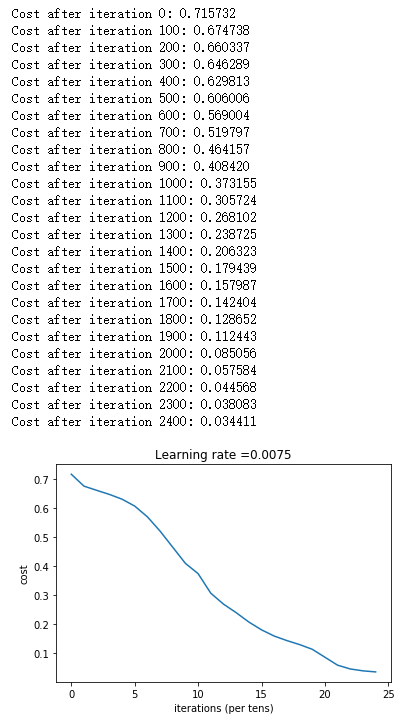
parameters = L_layer_model(train_x, train_y, layers_dims, num_iterations = 2500, print_cost = True)

得到如下运行结果：

此处与L4-1中函数def initialize_parameters_deep(layer_dims)有区别

原因在于不同激活函数使用的初始化方法是不同的

在给出参考中使用的初始化方法为tanh激活函数初始化方法：

w[l] = np.random.randn(n[l],n[l-1])*np.sqrt(1/n[l-1])

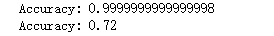
求模型的准确率：

pred_train = predict(train_x, train_y, parameters)
pred_test = predict(test_x, test_y, parameters)

结果如下所示：

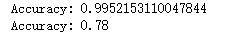
此处与原作业中结果仍不一致，原因未知，但整体为正确学习结果，因此不再进行追究

2.4 结果分析

针对L层标记错误的图像，下面代码将显示分类错误图像：

print_mislabeled_images(classes, test_x, test_y, pred_test)

得到如下运行结果：

该模型在表现效果较差的的图像包括：

猫身处于异常位置
图片背景与猫颜色类似
猫的种类和颜色稀有
相机角度
图片的亮度
比例变化（猫的图像很大或很小）

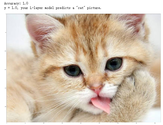
2.5 使用自己的图像进行测试

修改以下代码中图像的路径及标签：

# change this to the name of your image file 
my_image = "my_image.jpg"
# the true class of your image (1 -> cat, 0 -> non-cat)
my_label_y = [1] 

fname = my_image
image = np.array(plt.imread(fname))
my_image = np.array(Image.fromarray(image).resize(size=(num_px,num_px))).reshape((num_px*num_px*3,1))
my_predicted_image = predict(my_image, my_label_y, parameters)

plt.imshow(image)
print ("y = " + str(np.squeeze(my_predicted_image)) + ", your L-layer model predicts a \"" + classes[int(np.squeeze(my_predicted_image)),].decode("utf-8") +  "\" picture.")