视觉SLAM十四讲笔记-8-2

视觉SLAM十四讲笔记-8-2

8.4 直接法

8.4.1 直接法的推导

在光流中，会首先追踪特征点的位置，再根据这些位置确定相机的运动。这种两步走的方案，很难保证全局的最优性。那么能不能在后一步中，调整前一步的结果尼?例如，如果认为相机右转了 $15^{\circ }$，那么光流能不能以这个 $15^{\circ }$ 运动作为初始值的假设，调整光流的计算结果尼?直接法就是遵循这样的思路得到的结果。
如下图，图片链接:link，考虑某个空间点 $P$ 和两个时刻的相机。 $P$ 的世界坐标为 $[X,Y,Z]$，它在两个相机上的成像，记作像素坐标为 $p_1,p_2$。

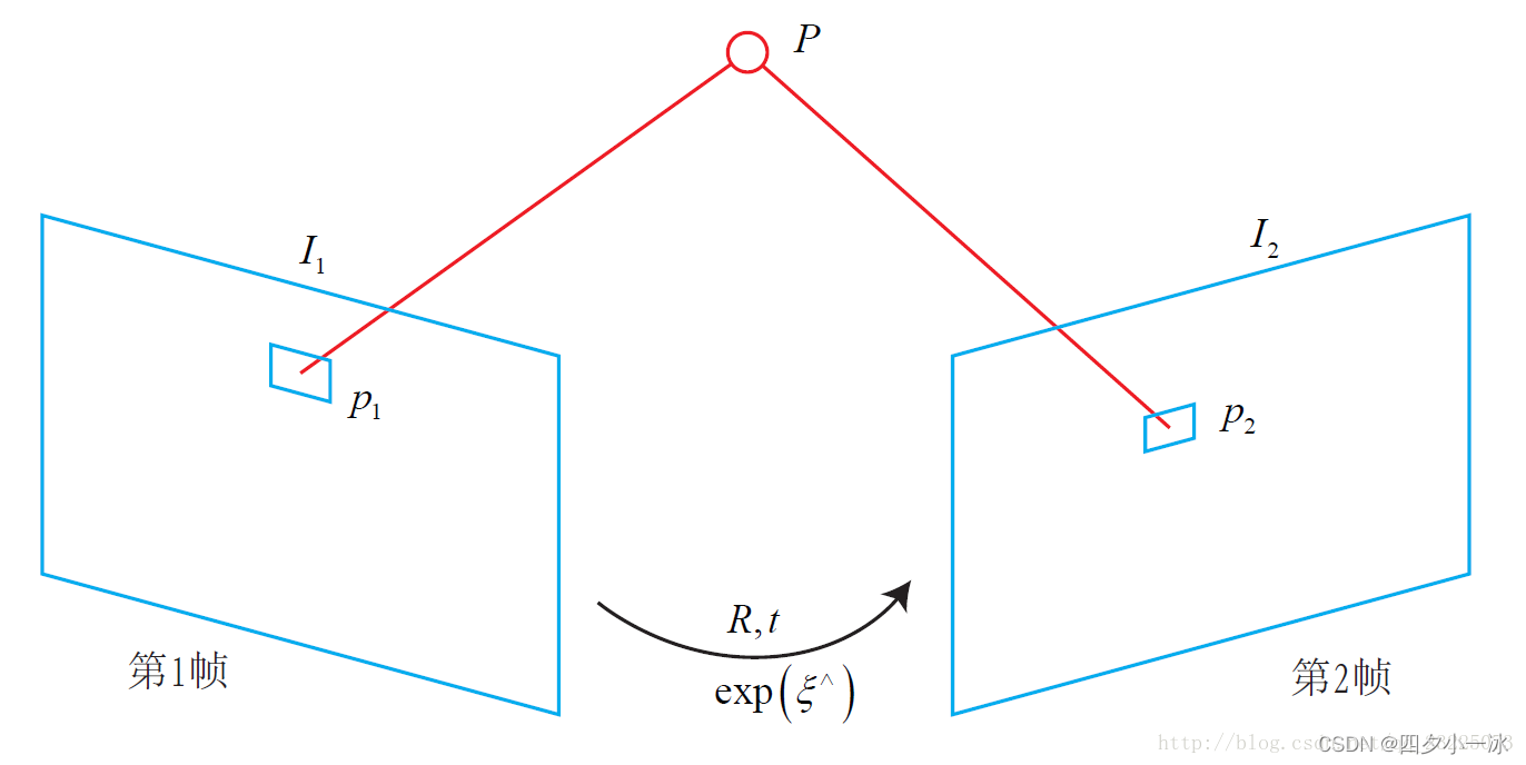
目标是要求第一个相机到第二个相机的相对位姿变换。以第一个相机为参照系，设第二个相机的旋转和平移为 $R,t$(对应的李群为 $T$)。同时，两相机的内参相同，记为 $K$。
$$\begin{array}{rl}& p_1={\left[\begin{array}{l}u\\ v\\ 1\end{array}\right]}_1=\frac{1}{Z_1}KP\\ & p_2={\left[\begin{array}{l}u\\ v\\ 1\end{array}\right]}_2=\frac{1}{Z_2}K(RP+t)=\frac{1}{Z_2}K(TP{)}_{1:3}\end{array}$$在特征点法中，由于通过匹配描述子知道了 $p_1,p_2$ 的像素位置，所以可以计算重投影的位置。但是，在直接法中，由于没有特征匹配，无法知道哪一个 $p_2$ 与 $p_1$ 对应着同一个点。直接法的思路是根据当前相机的位姿估计之寻找 $p_2$ 的位置。但若相机位姿不够好， $p_2$ 的外观和 $p_1$ 会有明显差别。于是，为了减少这个差别，通过优化相机的位姿来寻找与 $p_1$ 更相似的 $p_2$。这同样可以通过一个优化问题去完成，但此时最小化的不是重投影误差，而是光度误差，也就是 $P$ 的两个像素的亮度误差：
$$e=I_1(p_1)-I_2(p_2)$$这里的 $e$ 是一个标量。同样地，优化目标为该误差的二范数，暂时写成不加权的形式，为：
$$\underset{T}{\min }J(T)={\Vert e\Vert }^2$$能够做这种优化的理由，仍然是基于灰度不变假设。假设一个空间点在各个视角下成像灰度是不变的。若有许多个(比如 N 个) 空间点 $P_i$，那么，整个相机位姿估计问题变为：
$$\underset{T}{\min }J(T)=\sum _{i=1}^N{e}_i^T{e}_i,e_i={\mathbf{I}}_i\left({\mathbf{p}}_1,i\right)-{\mathbf{I}}_2\left({\mathbf{p}}_2,i\right)$$
注意，这里的优化变量是相机位姿 $T$，而不像光流那样优化各个特征点的运动。为了求解这个优化问题，关心误差 $e$ 是如何随着相机位姿 $T$ 变化的，需要分析其导数关系。因此，定义两个中间变量：
$$\begin{gathered} q=TP, \\ u=\frac{1}{Z_2}Kq \end{gathered}$$
这里的 $q$ 为 $P$ 在第二个相机坐标系下的坐标，而 $u$ 为它的像素坐标。显然 $q$ 是 $T$ 的函数，$u$ 是 $q$ 的函数，从而也是 $T$ 的函数。
考虑到李代数的左扰动模型，利用一节泰勒展开，因为：
$$e(T)=I_1(p_1)-I_2(u)$$所以：
$$\frac{\partial e}{\partial T}=\frac{\partial I_2}{\partial u}\frac{\partial u}{\partial q}\frac{\partial q}{\partial \delta \xi }\delta \xi$$其中，
$\delta \xi$ 为 $T$ 的左扰动。可以看到，一阶导数由于链式法则分成了 3 项，而这三项都是容易计算的：

1. $\frac{\partial I_2}{\partial u}$ 为 $u$ 处的梯度。

2. $\frac{\partial u}{\partial q}$ 为投影方程关于相机坐标系下的三维点的导数。记 $q=[X,Y,Z{]}^T$，
   $$\frac{\partial u}{\partial q}=-\left[\begin{array}{lll}\frac{\partial u}{\partial X}& \frac{\partial u}{\partial Y}& \frac{\partial u}{\partial Z}\\ \frac{\partial v}{\partial X}& \frac{\partial v}{\partial Y}& \frac{\partial v}{\partial Z}\end{array}\right]=-\left[\begin{array}{ccc}\frac{f_x}{Z}& 0& -\frac{f_{x}X}{Z^2}\\ 0& \frac{f_y}{Z}& -\frac{f_{y}Y}{Z^2}\end{array}\right]$$

3.$\frac{\partial q}{\partial \delta \xi }$ 为变换后的三维点对变换的导数，
而第二项为变换后关于李代数的导数。
$$\frac{\partial (q)}{\partial \delta \xi }=(TP{)}^{\odot }=\left[\begin{array}{cc}I& -q^{\wedge }\\ 0^T& 0^T\end{array}\right]$$
而在 $q$ 的定义中，取出了前 3 维，于是得：
$$\frac{\partial q}{\partial \delta \xi }=\left[I,-q^{\wedge }\right]=\left[\begin{array}{cccccc}1& 0& 0& 0& Z& -Y\\ 0& 1& 0& -Z& 0& X\\ 0& 0& 1& Y& -X& 0\end{array}\right]$$
将其两项相乘，就得到了 2 * 6 的雅克比矩阵：
$$\frac{\partial u}{\partial \delta \xi }=-\left[\begin{array}{cccccc}\frac{f_x}{Z}& 0& -\frac{f_{x}X}{Z^2}& -\frac{f_{x}XY}{Z^2}& f_x+\frac{f_x{X}^2}{Z^2}& -\frac{f_{x}Y}{Z}\\ & & & & & \\ 0& \frac{f_y}{Z}& -\frac{f_y{Y}^{\prime }}{Z^2}& -f_y-\frac{f_y{Y}^2}{Z^2}& \frac{f_{y}XY}{Z^2}& \frac{f_{y}X}{Z}\end{array}\right]$$
推导出误差对于李代数的雅克比矩阵：
$$J=\frac{\partial I_2}{\partial u}\frac{\partial u}{\partial \delta \xi }$$
对于 $N$ 个点的问题，可以用这种方法计算优化问题的雅克比矩阵，然后使用高斯牛顿法或者列文伯格-马夸尔特计算增量，迭代求解。至此，推导出了直接法估计相机位姿的整个流程。

8.4.2 直接法的讨论

在上面的讨论中，$P$ 是一个已知位置的空间点，它是怎么来的尼?在 RGB-D 相机中，可以把任意像素反投影到三维空间，然后再投影到下一幅图像中。如果在双目相机中，同样可以根据视差来计算像素的深度。如果在单目相机中，这件事情还比较困难，因为还需要考虑 $P$ 的深度带来的不确定性。
现在先来考虑 $P$ 深度已知的情况。根据 $P$ 的来源，将直接法进行分类：
1.$P$ 来源于稀疏关键点，称之为稀疏直接法。通常，使用数百个至上千个关键点，并且像 L-K 光流那样，假设它周围像素也是不变的。这种稀疏直接法不必计算描述子，并且只使用数百个像素，因此速度最快，但只能计算稀疏的重构。
2.$P$ 来自部分像素，从 $J=\frac{\partial I_2}{\partial u}\frac{\partial u}{\partial \delta \xi }$ 中可以看出，如果像素梯度为零，那么整项雅克比矩阵就为零，不会对计算运动增量有任何贡献。因此，可以考虑只使用带有梯度的像素点，舍弃像素梯度不明显的地方。这称为半稠密的直接法，可以重构一个半稠密结构。
3.$P$ 为所有像素，称为稠密直接法。稠密重构需要计算所有像素(一般几十万至几百万个)，因此多数不能在现有的 CPU 上实时计算，需要 GPU 的加速。但是，像素梯度不明显的点，在运动估计中不会有太大贡献，在重构时也会难以估计位置。
可以看到，从稀疏到稠密重构，都可以用直接法计算。它们的计算是逐渐增长的。稀疏方法可以快速地求解相机位姿，而稠密方法可以建立完整地图。具体使用哪种方法，需要视机器人的应用环境而定。

8.5 实践：直接法

8.5.1 单层直接法

求解直接法最后等价于求解一个优
化问题，因此可以使用 g2o 或者 Ceres 这些优化库来帮助求解，也可以自己实现高斯牛顿法。和光流类似，直接法也可以分为单层直接法和金字塔式的多层直接法。
在单层直接法中，类似于并行的光流，也可以并行地计算每个像素点的误差和雅克比，为此定义一个求雅克比的类：

mkdir direct_method
cd direct_method/
code .

//launch.json
{
    // Use IntelliSense to learn about possible attributes.
    // Hover to view descriptions of existing attributes.
    // For more information, visit: https://go.microsoft.com/fwlink/?linkid=830387
    "version": "0.2.0",
    "configurations": [
        {
            "name": "g++ - 生成和调试活动文件",
            "type": "cppdbg",
            "request":"launch",
            "program":"${workspaceFolder}/build/direct_method",
            "args": [],
            "stopAtEntry": false,
            "cwd": "${workspaceFolder}",
            "environment": [],
            "externalConsole": false,
            "MIMode": "gdb",
            "setupCommands": [
                {
                    "description": "为 gdb 启动整齐打印",
                    "text": "-enable-pretty-printing",
                    "ignoreFailures": true
                }
            ],
            "preLaunchTask": "Build",
            "miDebuggerPath": "/usr/bin/gdb"
        }
    ]
}

//tasks.json
{
	"version": "2.0.0",
	"options":{
		"cwd": "${workspaceFolder}/build"   //指明在哪个文件夹下做下面这些指令
	},
	"tasks": [
		{
			"type": "shell",
			"label": "cmake",   //label就是这个task的名字,这个task的名字叫cmake
			"command": "cmake", //command就是要执行什么命令,这个task要执行的任务是cmake
			"args":[
				".."
			]
		},
		{
			"label": "make",  //这个task的名字叫make
			"group": {
				"kind": "build",
				"isDefault": true
			},
			"command": "make",  //这个task要执行的任务是make
			"args": [

			]
		},
		{
			"label": "Build",
			"dependsOrder": "sequence", //按列出的顺序执行任务依赖项
			"dependsOn":[				//这个label依赖于上面两个label
				"cmake",
				"make"
			]
		}
	]
}

#CMakeLists.txt
cmake_minimum_required(VERSION 3.0)

project(DIRECTMETHOD)

#在g++编译时，添加编译参数，比如-Wall可以输出一些警告信息
set(CMAKE_CXX_FLAGS "${CMAKE_CXX_FLAGS} -Wall -std=c++14")

#一定要加上这句话，加上这个生成的可执行文件才是可以Debug的，不然不加或者是Release的话生成的可执行文件是无法进行调试的
set(CMAKE_BUILD_TYPE Debug)

list( APPEND CMAKE_MODULE_PATH /home/lss/Downloads/g2o/cmake_modules )
set(G2O_ROOT /usr/local/include/g2o)

# 为使用 sophus，需要使用find_package命令找到它
find_package(Sophus REQUIRED)
include_directories( ${Sophus_INCLUDE_DIRS} )

# Eigen
include_directories("/usr/include/eigen3")

find_package(Pangolin REQUIRED)
include_directories(${Pangolin_INCLUDE_DIRS})

find_package (glog 0.6.0 REQUIRED)


#此工程要调用opencv库，因此需要添加opancv头文件和链接库
#寻找OpenCV库
find_package(OpenCV REQUIRED)
#添加头文件
include_directories(${OpenCV_INCLUDE_DIRS})

# g2o
find_package(G2O REQUIRED)
include_directories(${G2O_INCLUDE_DIRS})

add_executable(direct_method direct_method.cpp)

#链接OpenCV库,Ceres库，
target_link_libraries(direct_method ${OpenCV_LIBS} ${G2O_CORE_LIBRARY} ${G2O_STUFF_LIBRARY} glog::glog)
target_link_libraries(direct_method Sophus::Sophus)
target_link_libraries(direct_method ${Pangolin_LIBRARIES})

#include <opencv2/opencv.hpp>
#include <sophus/se3.hpp>
#include <boost/format.hpp>
#include <pangolin/pangolin.h>
#include <mutex>
#include <algorithm>
#include <chrono>

using namespace std;

typedef vector<Eigen::Vector2d, Eigen::aligned_allocator<Eigen::Vector2d>> VecVector2d;

// Camera intrinsics相机内参
double fx = 718.856, fy = 718.856, cx = 607.1928, cy = 185.2157;
// baseline双目相机的基线
double baseline = 0.573;
// paths
string left_file = "./left.png";
string disparity_file = "./disparity.png";
boost::format fmt_others("./%06d.png");    // other files

// useful typedefs
typedef Eigen::Matrix<double, 6, 6> Matrix6d;
typedef Eigen::Matrix<double, 2, 6> Matrix26d;
typedef Eigen::Matrix<double, 6, 1> Vector6d;

/// class for accumulator jacobians in parallel
class JacobianAccumulator {
public:
    JacobianAccumulator(
        const cv::Mat &img1_,
        const cv::Mat &img2_,
        const VecVector2d &px_ref_, //角点坐标
        const vector<double> depth_ref_, //相机坐标系下的深度
        Sophus::SE3d &T21_) :
        img1(img1_), img2(img2_), px_ref(px_ref_), depth_ref(depth_ref_), T21(T21_) {
        projection = VecVector2d(px_ref.size(), Eigen::Vector2d(0, 0));
    }

    /// accumulate jacobians in a range 在 range 范围内加速计算雅克比矩阵
    void accumulate_jacobian(const cv::Range &range);

    /// get hessian matrix 获取海塞矩阵
    Matrix6d hessian() const { return H; }

    /// get bias 获取矩阵b
    Vector6d bias() const { return b; }

    /// get total cost 获取总共的代价
    double cost_func() const { return cost; }

    /// get projected points 获取图像2中的角点坐标
    VecVector2d projected_points() const { return projection; }

    /// reset h, b, cost to zero
    void reset() {
        H = Matrix6d::Zero();
        b = Vector6d::Zero();
        cost = 0;
    }

private:
    const cv::Mat &img1;
    const cv::Mat &img2;
    const VecVector2d &px_ref;
    const vector<double> depth_ref;
    Sophus::SE3d &T21;
    VecVector2d projection; // projected points

    std::mutex hessian_mutex;
    Matrix6d H = Matrix6d::Zero();
    Vector6d b = Vector6d::Zero();
    double cost = 0;
};

/**
 * pose estimation using direct method
 * @param img1
 * @param img2
 * @param px_ref
 * @param depth_ref
 * @param T21
 */
void DirectPoseEstimationMultiLayer(
    const cv::Mat &img1,
    const cv::Mat &img2,
    const VecVector2d &px_ref,
    const vector<double> depth_ref,
    Sophus::SE3d &T21
);

/**/
/*paths
string left_file = "./left.png";
 * pose estimation using direct method
 * @param img1
 * @param img2
 * @param px_ref
 * @param depth_ref
 * @param T21
 */
void DirectPoseEstimationSingleLayer(
    const cv::Mat &img1,
    const cv::Mat &img2,
    const VecVector2d &px_ref,
    const vector<double> depth_ref,
    Sophus::SE3d &T21
);

// bilinear interpolation
// bilinear interpolation
//使用双线性内插法来估计一个点的像素：
//f(x,y) \approx f(0,0)(1-x)(1-y) + f(1,0)x(1-y)+f(0,1)(1-x)y + f(1,1)xy
inline float GetPixelValue(const cv::Mat &img, float x, float y) {
    // boundary check
    if (x < 0) x = 0;
    if (y < 0) y = 0;
    if (x >= img.cols) x = img.cols - 1;
    if (y >= img.rows) y = img.rows - 1;
    uchar *data = &img.data[int(y) * img.step + int(x)];
    float xx = x - floor(x);
    float yy = y - floor(y);
    return float(
        (1 - xx) * (1 - yy) * data[0] +
        xx * (1 - yy) * data[1] +
        (1 - xx) * yy * data[img.step] +
        xx * yy * data[img.step + 1]
    );
}

int main(int argc, char **argv) {

    cv::Mat left_img = cv::imread(left_file, 0);
    cv::Mat disparity_img = cv::imread(disparity_file, 0);

    // let's randomly pick pixels in the first image and generate some 3d points in the first image's frame
    cv::RNG rng;
    int nPoints = 2000;
    int boarder = 20;
    VecVector2d pixels_ref;
    vector<double> depth_ref;

    // generate pixels in ref and load depth data
    //随机生成一些点并获取其像素位置和深度信息
    for (int i = 0; i < nPoints; i++) {
        int x = rng.uniform(boarder, left_img.cols - boarder);  // don't pick pixels close to boarder
        int y = rng.uniform(boarder, left_img.rows - boarder);  // don't pick pixels close to boarder
        int disparity = disparity_img.at<uchar>(y, x);
        double depth = fx * baseline / disparity; // you know this is disparity to depth//双目相机计算深度公式
        depth_ref.push_back(depth);
        pixels_ref.push_back(Eigen::Vector2d(x, y));
    }

    // estimates 01~05.png's pose using this information
    Sophus::SE3d T_cur_ref;

    for (int i = 1; i < 6; i++) {  // 1~10
        cv::Mat img = cv::imread((fmt_others % i).str(), 0);
        // try single layer by uncomment this line
         DirectPoseEstimationSingleLayer(left_img, img, pixels_ref, depth_ref, T_cur_ref);
        //DirectPoseEstimationMultiLayer(left_img, img, pixels_ref, depth_ref, T_cur_ref);
    }
    return 0;
}

void DirectPoseEstimationSingleLayer(
    const cv::Mat &img1,
    const cv::Mat &img2,
    const VecVector2d &px_ref, //img1中的像素坐标
    const vector<double> depth_ref, //像素坐标对应的深度
    Sophus::SE3d &T21) {

    const int iterations = 10; //设置迭代次数为 10
    double cost = 0, lastCost = 0;
    auto t1 = chrono::steady_clock::now();
    JacobianAccumulator jaco_accu(img1, img2, px_ref, depth_ref, T21);

    for (int iter = 0; iter < iterations; iter++) {
        jaco_accu.reset(); //重置
        //完成并行计算海塞矩阵H，矩阵b和代价cost
        cv::parallel_for_(cv::Range(0, px_ref.size()),
                          std::bind(&JacobianAccumulator::accumulate_jacobian, &jaco_accu, std::placeholders::_1));
        Matrix6d H = jaco_accu.hessian(); //计算海塞矩阵
        Vector6d b = jaco_accu.bias(); //计算b矩阵

        // solve update and put it into estimation
        Vector6d update = H.ldlt().solve(b);;
        T21 = Sophus::SE3d::exp(update) * T21;
        cost = jaco_accu.cost_func();

        if (std::isnan(update[0])) {
            // sometimes occurred when we have a black or white patch and H is irreversible
            cout << "update is nan" << endl;
            break;
        }
        if (iter > 0 && cost > lastCost) {
            cout << "cost increased: " << cost << ", " << lastCost << endl;
            break;
        }
        if (update.norm() < 1e-3) {
            // converge
            break;
        }

        lastCost = cost;
        cout << "iteration: " << iter << ", cost: " << cost << endl;
    }

    cout << "T21 = \n" << T21.matrix() << endl;
    auto t2 = chrono::steady_clock::now();
    auto time_used = chrono::duration_cast<chrono::duration<double>>(t2 - t1);
    cout << "direct method for single layer: " << time_used.count() << endl;

    // plot the projected pixels here
    cv::Mat img2_show;
    cv::cvtColor(img2, img2_show, CV_GRAY2BGR);
    VecVector2d projection = jaco_accu.projected_points();
    for (size_t i = 0; i < px_ref.size(); ++i) {
        auto p_ref = px_ref[i];
        auto p_cur = projection[i];
        if (p_cur[0] > 0 && p_cur[1] > 0) {
            cv::circle(img2_show, cv::Point2f(p_cur[0], p_cur[1]), 2, cv::Scalar(0, 250, 0), 2);
            cv::line(img2_show, cv::Point2f(p_ref[0], p_ref[1]), cv::Point2f(p_cur[0], p_cur[1]),
                     cv::Scalar(0, 250, 0));
        }
    }
    cv::imshow("current", img2_show);
    cv::waitKey();
}

void JacobianAccumulator::accumulate_jacobian(const cv::Range &range) {

    // parameters
    const int half_patch_size = 1;
    int cnt_good = 0;
    Matrix6d hessian = Matrix6d::Zero();
    Vector6d bias = Vector6d::Zero();
    double cost_tmp = 0;

    for (size_t i = range.start; i < range.end; i++) {

        // compute the projection in the second image
        //point_ref表示img1中的像素点，point_ref为其相机坐标系下的点
        Eigen::Vector3d point_ref =
            depth_ref[i] * Eigen::Vector3d((px_ref[i][0] - cx) / fx, (px_ref[i][1] - cy) / fy, 1);
        //计算在第二个图像对应的相机坐标系下的坐标
        Eigen::Vector3d point_cur = T21 * point_ref;
        if (point_cur[2] < 0)   // depth invalid
            continue;
        //将其转化到第二幅图像对应的像素坐标系下
        float u = fx * point_cur[0] / point_cur[2] + cx, v = fy * point_cur[1] / point_cur[2] + cy;
        if (u < half_patch_size || u > img2.cols - half_patch_size || v < half_patch_size ||
            v > img2.rows - half_patch_size)
            continue;

        projection[i] = Eigen::Vector2d(u, v);
        double X = point_cur[0], Y = point_cur[1], Z = point_cur[2],
            Z2 = Z * Z, Z_inv = 1.0 / Z, Z2_inv = Z_inv * Z_inv;
        cnt_good++;

        // and compute error and jacobian
        for (int x = -half_patch_size; x <= half_patch_size; x++)
            for (int y = -half_patch_size; y <= half_patch_size; y++) {

                double error = GetPixelValue(img1, px_ref[i][0] + x, px_ref[i][1] + y) -
                               GetPixelValue(img2, u + x, v + y);
                Matrix26d J_pixel_xi;
                Eigen::Vector2d J_img_pixel;

                J_pixel_xi(0, 0) = fx * Z_inv;
                J_pixel_xi(0, 1) = 0;
                J_pixel_xi(0, 2) = -fx * X * Z2_inv;
                J_pixel_xi(0, 3) = -fx * X * Y * Z2_inv;
                J_pixel_xi(0, 4) = fx + fx * X * X * Z2_inv;
                J_pixel_xi(0, 5) = -fx * Y * Z_inv;

                J_pixel_xi(1, 0) = 0;
                J_pixel_xi(1, 1) = fy * Z_inv;
                J_pixel_xi(1, 2) = -fy * Y * Z2_inv;
                J_pixel_xi(1, 3) = -fy - fy * Y * Y * Z2_inv;
                J_pixel_xi(1, 4) = fy * X * Y * Z2_inv;
                J_pixel_xi(1, 5) = fy * X * Z_inv;

                J_img_pixel = Eigen::Vector2d(
                    0.5 * (GetPixelValue(img2, u + 1 + x, v + y) - GetPixelValue(img2, u - 1 + x, v + y)),
                    0.5 * (GetPixelValue(img2, u + x, v + 1 + y) - GetPixelValue(img2, u + x, v - 1 + y))
                );//dx,dy是优化变量 即（Δu，Δv） 计算雅克比矩阵

                // total jacobian
                Vector6d J = -1.0 * (J_img_pixel.transpose() * J_pixel_xi).transpose();

                hessian += J * J.transpose();
                bias += -error * J;
                cost_tmp += error * error;
            }
    }

    if (cnt_good) {
        // set hessian, bias and cost
        unique_lock<mutex> lck(hessian_mutex);
        H += hessian;
        b += bias;
        cost += cost_tmp / cnt_good;
    } //cost = || eij ||2 2范数
}

void DirectPoseEstimationMultiLayer(
    const cv::Mat &img1,
    const cv::Mat &img2,
    const VecVector2d &px_ref,
    const vector<double> depth_ref,
    Sophus::SE3d &T21) {

    // parameters
    int pyramids = 4;
    double pyramid_scale = 0.5;
    double scales[] = {1.0, 0.5, 0.25, 0.125};

    // create pyramids
    vector<cv::Mat> pyr1, pyr2; // image pyramids
    for (int i = 0; i < pyramids; i++) {
        if (i == 0) {
            pyr1.push_back(img1);
            pyr2.push_back(img2);
        } else {
            cv::Mat img1_pyr, img2_pyr;
            cv::resize(pyr1[i - 1], img1_pyr,
                       cv::Size(pyr1[i - 1].cols * pyramid_scale, pyr1[i - 1].rows * pyramid_scale));
            cv::resize(pyr2[i - 1], img2_pyr,
                       cv::Size(pyr2[i - 1].cols * pyramid_scale, pyr2[i - 1].rows * pyramid_scale));
            pyr1.push_back(img1_pyr);
            pyr2.push_back(img2_pyr);
        }
    }

    double fxG = fx, fyG = fy, cxG = cx, cyG = cy;  // backup the old values
    for (int level = pyramids - 1; level >= 0; level--) {
        VecVector2d px_ref_pyr; // set the keypoints in this pyramid level
        for (auto &px: px_ref) {
            px_ref_pyr.push_back(scales[level] * px);
        }

        // scale fx, fy, cx, cy in different pyramid levels
        fx = fxG * scales[level];
        fy = fyG * scales[level];
        cx = cxG * scales[level];
        cy = cyG * scales[level];
        DirectPoseEstimationSingleLayer(pyr1[level], pyr2[level], px_ref_pyr, depth_ref, T21);
    }

}

运行结果：






从原始图片中随机生成的一些点，不使用任何角点或特征点提取算法，然后对 000001.png-000005.png 这五张图像，利用直接法计算相机的位姿。

8.5.2 多层直接法

然后类似于光流，再把单层直接法拓展到金字塔式的多层直接法上，用 Coarse-to-fine 的过程计算相对运动。
需要注意的是，直接法求雅克比的时候带上了内参，而当金字塔对图像进行缩放时，对应的内参也需要乘以相应的倍率。
只需要在上述程序中将 main 函数中改一下。

for (int i = 1; i < 6; i++) {  // 1~10
        cv::Mat img = cv::imread((fmt_others % i).str(), 0);
        // try single layer by uncomment this line
         //DirectPoseEstimationSingleLayer(left_img, img, pixels_ref, depth_ref, T_cur_ref);
        DirectPoseEstimationMultiLayer(left_img, img, pixels_ref, depth_ref, T_cur_ref);
    }

从运行结果可以看出，即使随机选点，直接法也能够正确追踪大部分的像素，同时估计相机的运动。这中间没有任何的特征提取、匹配或者光流的过程。从运行时间也可以看出，在 2000 个点时，直接法每迭代一层需要 1-2 毫秒，所以四层金字塔约耗时 8 毫秒。相比之下，2000 个点的光流耗时大约在十几毫秒，还不包括后续的位姿估计。所以，直接法相比于传统的特征点和光流通常更快一些。
相比于特征点法，直接法完全依靠优化来求解相机位姿。像素梯度引导着优化的方向。如果想要得到正确的优化结果，就必须保证大部分像素梯度能够把优化方向引导到正确的方向。

假设对于参考图像，我们测量到一个灰度值为 229 的像素。并且，由于深度已知，可以推断出空间点 $P$ 的位置（如下图所示，在 $I_1$ 中测量得到的灰度）。此时，我们又得到一幅新的图像，需要顾及它的相机位姿。这个位姿是由一个初值不断优化迭代得到的。假设我们的初值比较差，在这个初值下，空间点 $P$ 投影后的像素灰度值是 126。于是此像素的误差为 229-126=103。为了减小这个误差，我们希望微调相机的位姿，使得像素更亮一些。　
图片来源：link

怎么知道往哪里微调会更亮尼? 这需要用到局部的像素梯度。从图像中可以看到，沿着 $u$ 轴往前走一步，即减去了 3。同样地，沿着 $v$ 轴往前走一步，灰度值减去了 18。在这个像素周围，看到了梯度 $[-3,-18]$。为了提高亮度，会建议优化算法微调相机，使得 $P$ 的像素往左上方移动。在这个过程中，用像素的局部梯度近似了它附近的灰度分布，不过真是图像并不是光滑的，所以这个梯度在远处就不成立了。
但是，优化算法不能只看这一个像素，还需要听取其他像素的建议。综合听取了许多像素的意见之后，优化算法选择了一个和建议方向偏离不远的地方，计算一个新的更新量 $e^{{\xi }^{\wedge }}$。加上更新量后，图像从 $I_2$ 变成了 $I_2^{\prime }$，像素的投影位置也变到了一个更亮的地方。通过这次更新，误差变小了。在理想情况下，期望误差不断下降，最后收敛。
但是，实际上是否真的只要沿着梯度方向走，就能走到一个最优值尼?注意，直接法的梯度是直接由图像梯度确定的，因此必须保证沿着图像的梯度走时，灰度误差会不断下降。然而，图像通常是一个很强烈的非凸函数，实际中，如果沿着图像梯度前进，很容易由于图像的非凸性落进一个局部极小值中，无法继续优化。只有当相机运动很小时，图像中的梯度有很强的非凸性时，直接法才能成立。
图片来源：link

在例程中，只计算了单个像素的差异，并且差异是由灰度值直接相减得到的。然而，单个像素没有什么区分性，周围很可能有很多像素和它的亮度差不多。所以，有时会使用小的图像块 (patch)，并且使用更加复杂的度量形式，例如归一化相关性(Normalized Cross Correlation, NCC)等。

8.5.3 直接法的优缺点总结

直接法的优点：
1.可以省去计算特征点、描述子的时间。
2.只要求有像素梯度即可，不需要特征点。因此，直接法可以在特征缺失的场合下使用。比较极端的例子是只有渐变的一幅图像。他可能无法提取角点类特征，但可以用直接法估计它的运动。在演示实验中，直接法对随机选点也能正常工资。这一点实际使用中非常关键，因为实际场景很有可能没有很多角点可供使用。
3.可以构建半稠密乃至稠密的地图，这是特征点法无法做到的。

直接法的缺点也非常明显：
1.非凸性。直接法完全依赖于梯度搜索，降低目标函数来计算相机位姿。其目标函数中需要取像素点的灰度值，而图像是强烈非凸的函数。这使得优化算法容易进入极小值，只在运动很小时直接法才能成功。针对于此，金字塔的引入可以在一定程度上减小非凸性的影响。
2.单一像素没有区分度。和它像的实在太多了。于是我们要么计算图像块，要么计算复杂的相关性。由于每个像素对改变相机运动的意见不一致，只能少数服从多数，以数量代替质量。所以直接法在选点较少时的表现下降明显，通常建议用至少500个点以上。
3.灰度不变假设是很强的假设。如果相机是自动曝光的，当它调整曝光参数时，会使得图像整体变量或者变暗。光照变化时也会出现这种情况。特征点法对光照具有一定的容忍性，而直接法由于计算灰度间的差异，整体灰度变化会破坏灰度不变假设，使得算法失败。针对这一点，实用的直接法会同时估计相机的曝光参数，以便在曝光时间变化时也能工作。