


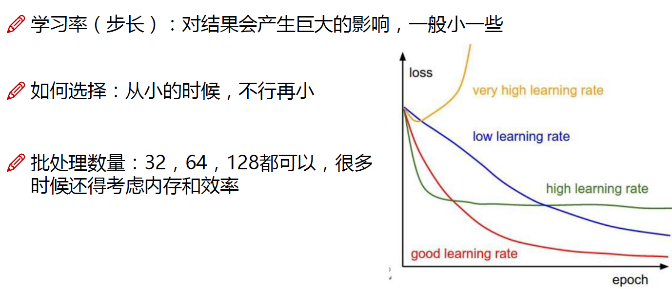
 本文介绍了线性回归的基本思想,如何通过梯度下降优化算法最小化误差,以及如何在Python中实现线性回归模型。通过GDP与幸福指数的关系实例,展示了如何训练模型并进行预测。
声明:此笔记仅作为记录使用,以免日后忘记,侵删,课程来源唐宇迪机器学习
目录
1.基本思想
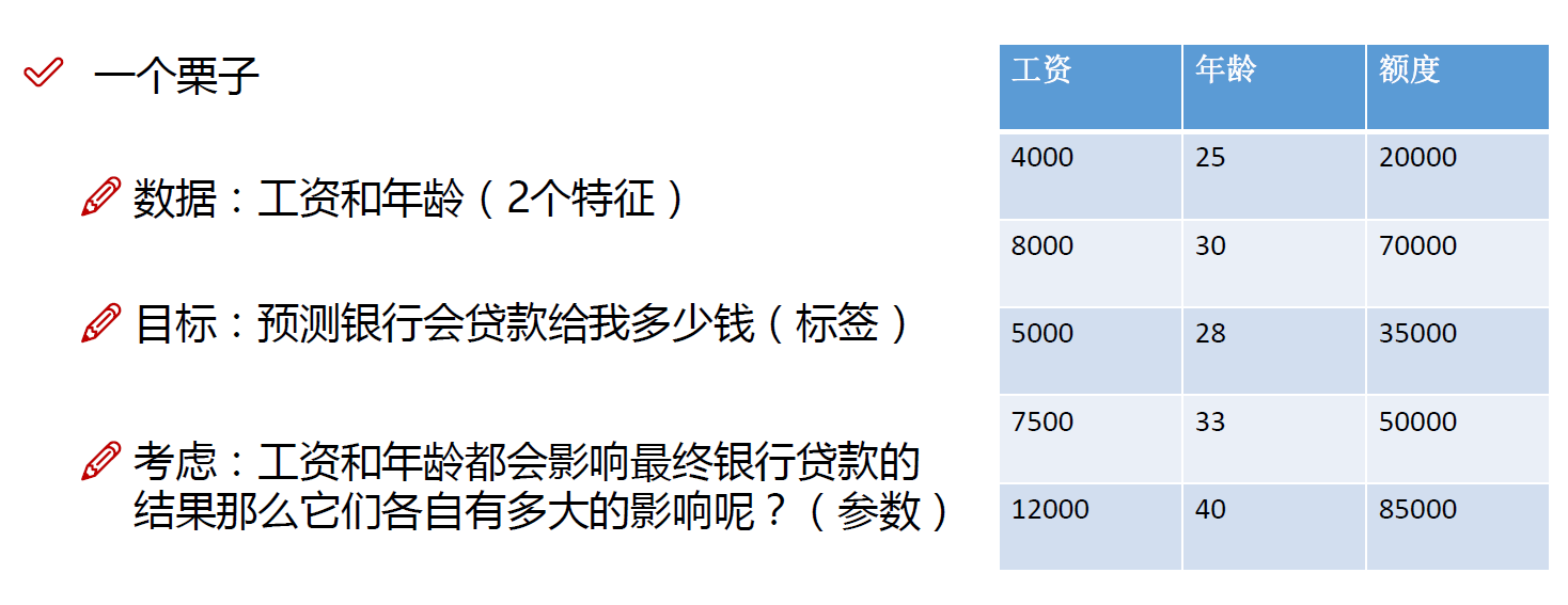
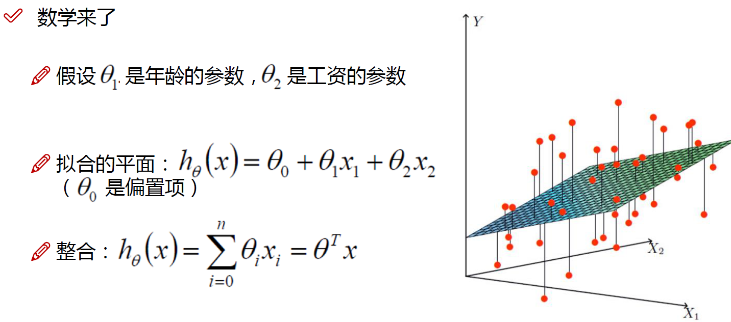
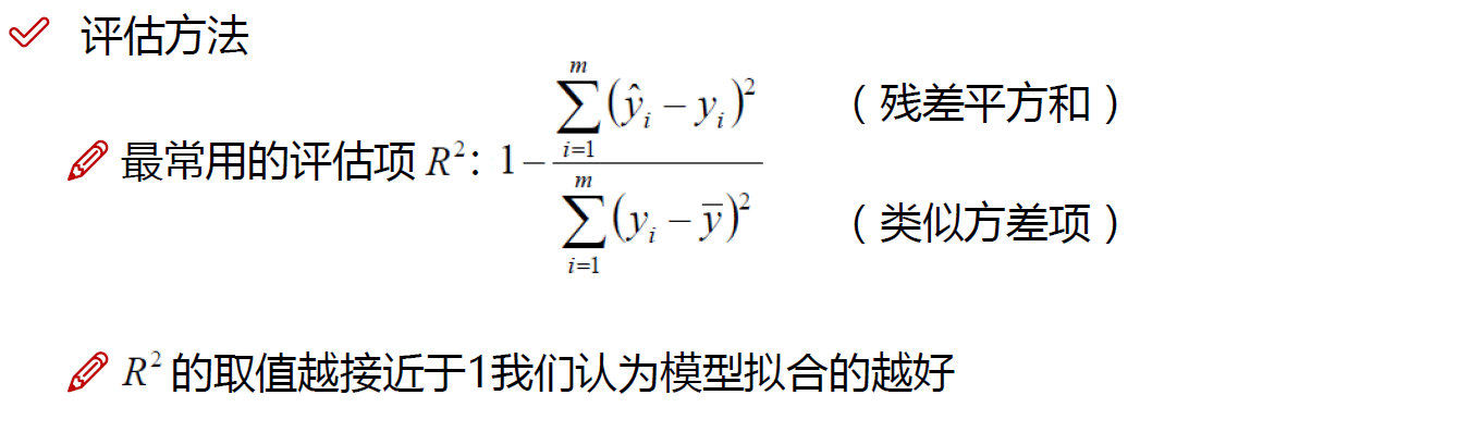
线性回归是机器学习中一种基本的监督学习算法,用于建模自变量(特征)与因变量(目标)之间的线性关系。其目标是找到一条直线,使得预测值与实际值的差异最小化。
2.例子

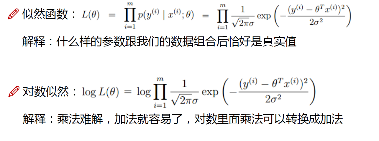
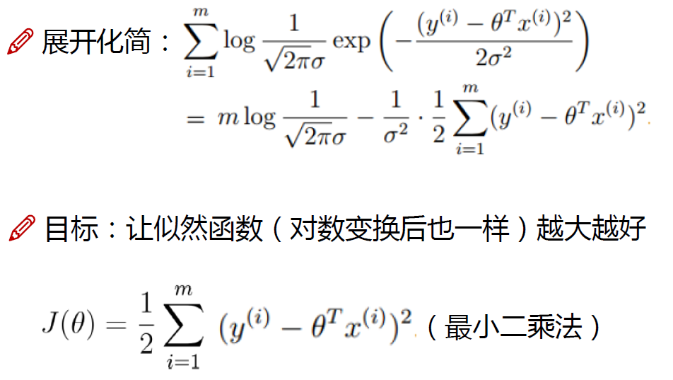
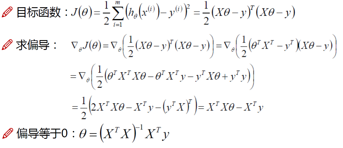
3.误差


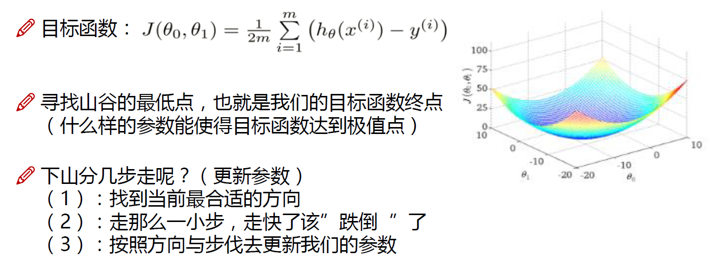
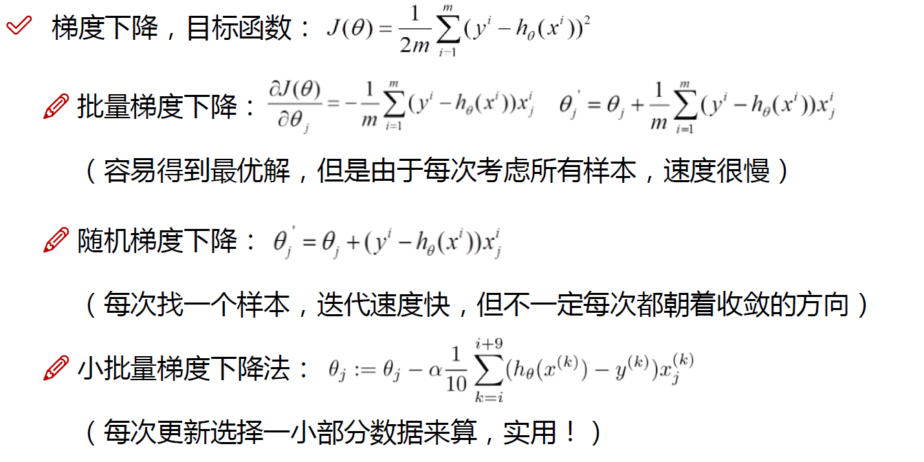
3.梯度下降
梯度下降是一种优化算法,常用于机器学习中的模型训练。它的主要目标是最小化(或最大化)一个目标函数,通过迭代调整模型参数,使得目标函数的值达到最小(或最大)。在机器学习中,常见的目标是最小化损失函数,即模型预测值与真实值之间的差异。梯度下降的优点有:
-
寻找全局最优解: 梯度下降能够帮助模型找到目标函数的局部最小值。虽然并非所有问题都有唯一的全局最优解,但梯度下降通常能够在参数空间中找到一个较好的解。
-
迭代更新: 梯度下降是一个迭代的过程,通过不断迭代更新模型参数,逐渐接近最优解。这种迭代的过程使得模型可以逐步提升性能。
4.代码
4.1线性回归模块
1.初始化对数据进行预处理
2.实现梯度下降
3.损失和预测模块
import numpy as np
from utils.features import prepare_for_training

class LinearRegression:

    def __init__(self,data,labels,polynomial_degree = 0,sinusoid_degree = 0,normalize_data=True):
        """
        1.对数据进行预处理操作
        2.先得到所有的特征个数
        3.初始化参数矩阵
        """
        (data_processed,
         features_mean,
         features_deviation)  = prepare_for_training(data, polynomial_degree, sinusoid_degree,normalize_data=True)

        self.data = data_processed
        self.labels = labels
        self.features_mean = features_mean
        self.features_deviation = features_deviation
        self.polynomial_degree = polynomial_degree
        self.sinusoid_degree = sinusoid_degree
        self.normalize_data = normalize_data

        num_features = self.data.shape[1]
        self.theta = np.zeros((num_features,1))

    def train(self,alpha,num_iterations = 500):
        """
                    训练模块,执行梯度下降
        """
        cost_history = self.gradient_descent(alpha,num_iterations)
        return self.theta,cost_history

    def gradient_descent(self,alpha,num_iterations):
        """
                    实际迭代模块,会迭代num_iterations次
        """
        cost_history = []
        for _ in range(num_iterations):
            self.gradient_step(alpha)
            cost_history.append(self.cost_function(self.data,self.labels))
        return cost_history


    def gradient_step(self,alpha):
        """
                    梯度下降参数更新计算方法,注意是矩阵运算
        """
        num_examples = self.data.shape[0]
        prediction = LinearRegression.hypothesis(self.data,self.theta)
        delta = prediction - self.labels
        theta = self.theta
        theta = theta - alpha*(1/num_examples)*(np.dot(delta.T,self.data)).T
        self.theta = theta


    def cost_function(self,data,labels):
        """
                    损失计算方法
        """
        num_examples = data.shape[0]
        delta = LinearRegression.hypothesis(self.data,self.theta) - labels
        cost = (1/2)*np.dot(delta.T,delta)/num_examples
        return cost[0][0]


    @staticmethod
    def hypothesis(data,theta):
        predictions = np.dot(data,theta)
        return predictions

    def get_cost(self,data,labels):
        data_processed = prepare_for_training(data,
         self.polynomial_degree,
         self.sinusoid_degree,
         self.normalize_data
         )[0]

        return self.cost_function(data_processed,labels)
    def predict(self,data):
        """
                    用训练的参数模型,与预测得到回归值结果
        """
        data_processed = prepare_for_training(data,
         self.polynomial_degree,
         self.sinusoid_degree,
         self.normalize_data
         )[0]

        predictions = LinearRegression.hypothesis(data_processed,self.theta)

        return predictions
4.2训练与预测
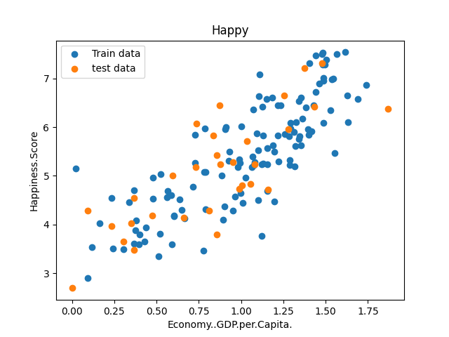
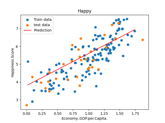
对GDP和幸福指数关系建立模型,并进行预测
import numpy as np
import pandas as pd
import matplotlib.pyplot as plt

from linear_regression import LinearRegression

data = pd.read_csv('../data/world-happiness-report-2017.csv')

# 得到训练和测试数据
train_data = data.sample(frac = 0.8)
test_data = data.drop(train_data.index)

input_param_name = 'Economy..GDP.per.Capita.'
output_param_name = 'Happiness.Score'

x_train = train_data[[input_param_name]].values
y_train = train_data[[output_param_name]].values

x_test = test_data[input_param_name].values
y_test = test_data[output_param_name].values

plt.scatter(x_train,y_train,label='Train data')
plt.scatter(x_test,y_test,label='test data')
plt.xlabel(input_param_name)
plt.ylabel(output_param_name)
plt.title('Happy')
plt.legend()
plt.show()

num_iterations = 500
learning_rate = 0.01

linear_regression = LinearRegression(x_train,y_train)
(theta,cost_history) = linear_regression.train(learning_rate,num_iterations)

print ('开始时的损失:',cost_history[0])
print ('训练后的损失:',cost_history[-1])

plt.plot(range(num_iterations),cost_history)
plt.xlabel('Iter')
plt.ylabel('cost')
plt.title('GD')
plt.show()

predictions_num = 100
x_predictions = np.linspace(x_train.min(),x_train.max(),predictions_num).reshape(predictions_num,1)
y_predictions = linear_regression.predict(x_predictions)

plt.scatter(x_train,y_train,label='Train data')
plt.scatter(x_test,y_test,label='test data')
plt.plot(x_predictions,y_predictions,'r',label = 'Prediction')
plt.xlabel(input_param_name)
plt.ylabel(output_param_name)
plt.title('Happy')
plt.legend()
plt.show()
训练和测试绘制训练和测试数据的散点图,80%是训练数据,20%是测试数据,设置梯度下降的迭代次数500次和学习率0.01。
绘制损失随着迭代次数变化的图表,以可视化梯度下降算法的收敛过程

预测并绘制预测线


 1万+
1万+


 被折叠的 条评论
为什么被折叠?
被折叠的 条评论
为什么被折叠?
 到【灌水乐园】发言


