Attention总结

Attention总结

对论文NML的总结，论文标题：

NEURAL MACHINE TRANSLATION BY JOINTLY LEARNING TO ALIGN AND TRANSLATE

算是attention的开山之作了。

这篇论文引出的Attention model（在论文中被称为alignment model），是依附于RNN Encoder-Decoder架构的。所以作者先对最基本的RNN Encoder-Decoder框架做了一个简单的介绍。

RNN Encoder-Decoder

an encoder reads the input sentence, a sequence of vectors $\mathbf{x}=(x_1,...,x_{T_x})$，into a vector $c$。其中我们记$\mathbf{x}$为source sentence，$x_i$ is 1-of-K coded word vector，$T_x$表示source sentence的长度。

对于RNN，
h t = f ( x t , h t − 1 ) c = q ( { h 1 , . . . , h T x } ) h_t = f(x_t, h_{t-1})\\c = q(\{h_1,...,h_{T_x}\}) ht​=f(xt​,ht−1​)c=q({h1​,...,hTx​​})
其中，$h_t$是时刻$t$的hidden state，$f$ and $g$ are some nonlinear functions。

the decoder is often trained to predict the next word $y_{t^{\prime }}$ given the context vector $c$ and all the
previously predicted words $y_1,...,y_{t^{\prime }-1}$。In other words, the decoder defines a probability over
the translation y by decomposing the joint probability into the ordered conditionals:
p ( y ) = ∏ t = 1 T y p ( y t ∣ { y 1 , . . . , y t − 1 } , c ) y = ( y 1 , . . . , y T y ) p(\bold{y}) = \prod_{t=1}^{T_y}p(y_t|\{y_1,...,y_{t-1}\},c)\\\bold{y} = (y_1, ...,y_{T_y}) p(y)=t=1∏Ty​​p(yt​∣{y1​,...,yt−1​},c)y=(y1​,...,yTy​​)
With an RNN, each conditional probability is modeled as
p ( y t ∣ { y 1 , . . . , y t − 1 } , c ) = g ( y t − 1 , s t , c ) p(y_t|\{y_1,...,y_{t-1}\},c) = g(y_{t-1}, s_t,c) p(yt​∣{y1​,...,yt−1​},c)=g(yt−1​,st​,c)
其中，$y_{t-1}$是上一时刻的输出，$s_t$是时刻t的hidden state，$g$是nonlinear function，可以是RNN或者LSTM单元。

当然，这里的RNN可以换成LSTM，并且效果会更好。

可以看出，无论是在联合概率表达式还是在单个的条件概率表达式中，context vector $c$都是相同的，即所谓的“分心模型”，从而引出后文的alignment model。

alignment model

在介绍这个model时，作者是以BiRNN为例。

在引入alignment model后，上一节定义的each conditional probability变成了：
$$p(y_i|y_1,...,y_{i-1},\mathbf{x})=g(y_{i-1},s_i,c_i)$$
$s_i$的更新表达式（$i$时刻的hidden state）：
$$s_i=f(s_{i-1},y_{i-1},c_i)$$
可以看出，$s_i$的更新表达式和常规RNN和LSTM形式差不多，只不过多了一个输入$c_i$。

这两个表达式的关键在于decoder在不同的时刻$c_i$也是不同的，即search through a source sentence $\mathbf{x}$ during decoding a translation to form $c_i$，而不是像上一节的表达式中不同时刻的$c$都是相同的。

下图是注意力分配的可视化计算过程：

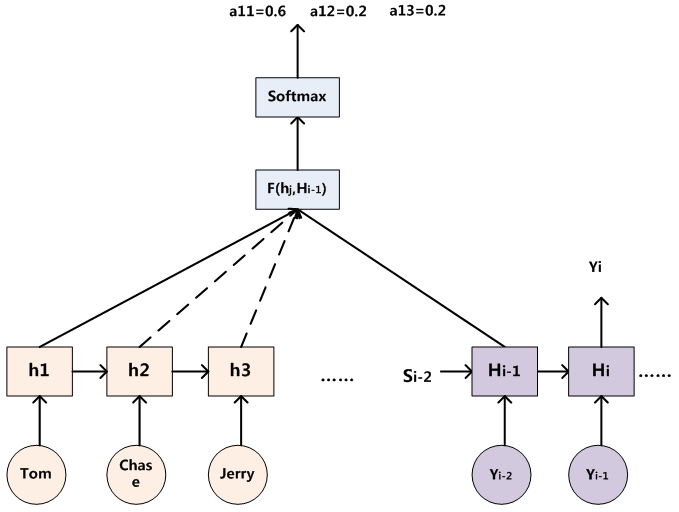
接下来看看如何计算context vector $c_i$：
$$\begin{gathered} c_i=\sum _{j=1}^{T_x}{\alpha }_{ij}{h}_j \\ {\alpha }_{ij}=\frac{exp(e_{ij})}{{\sum }_{k=1}^{T_x}exp(e_{ik})} \\ {e}_{ij}=a(s_{i-1},h_j) \end{gathered}$$
以上三个表达式就是所谓的alignment model（即我们现在所熟悉的attention机制）。为什么原文叫做alignment呢？scores how well the inputs around position $j$ and the output at position $i$ match。

可视化：

这里的AM其实是soft AM，意思是在求注意力分配概率分布的时候，对于source sentence $\mathbf{x}$中任意一个单词都给出一个对齐概率（即目标单词有多大可能是由当前这个单词decode得到，这就是对齐的意思），是一个概率分布。既然有soft AM，相应的也有hard AM，这里按下不表。

论文中AM is a feedforward neural network which is jointly trained with all the other components of the proposed system。具体形式为：
$$a(s_{i-1},h_j)={\mathbf{v}}_a^{T}tanh(W_a{s}_{i-1}+U_a{h}_j)$$

实际应用中注意力函数有很多变体。主流的注意力函数有：加性注意力（additive attention）、乘法（点积）注意力（multiplicative attention）、自注意力（self-attention）、键-值注意力（key-value attention）

additive attention:

来自于论文：Attention-Based Models for Speech Recognition。
$$\begin{gathered} f_{att}(h_i,s_{j-1})={\mathbf{v}}_a^{T}tanh(W_a[h_i;s_{j-1}]),i.e. \\ {f}_{att}(h_i,s_{j-1})={\mathbf{v}}_a^{T}tanh(W_1{h}_i+W_2{s}_{j-1}) \end{gathered}$$
本质是利用前馈网络来计算注意力分配。

multiplicative attention:

来自于论文：Effective Approaches to Attention-based Neural Machine Translation
$$f_{att}(h_i,s_{j-1})=h_i^T{W}_a{s}_{j-1}$$
加性注意力和乘法注意力在复杂度上是差不多的，但是乘法注意力在实践中更快、存储更高效，因为可以使用矩阵操作。

self-attention:

来自于论文：Attention is All you Need
$$\begin{gathered} A=softmax(V_{a}tanh(W_a{H}^T)) \\ C=AH \end{gathered}$$
自注意力和一般的注意力区别还是挺大的，所以这里的表达式没有涉及到$s_i$。Transformer是自注意力的典型应用。

key-value attention:

来自于论文：Frustratingly Short Attention Spans in Neural Language Modeling

这种注意力的计算方式的关键在于将$h_i$分离成一个键值$k_i$向量和一个值向量$v_i$，即$[k_i;v_i]=h_i$：
$$\begin{gathered} a_i=softmax({\mathbf{V}}_a^{T}tanh(W_1[{\mathbf{k}}_{i-L};,,,;{\mathbf{k}}_{i-1}]+(W_2{\mathbf{k}}_i)1^T)) \\ {c}_i=[{\mathbf{v}}_{i-L};,,,;{\mathbf{v}}_{i-1}]{\mathbf{a}}^T \\ \mathbf{c}=[\mathbf{c};v_i] \end{gathered}$$
$L$为注意力窗口的长度.

作者是以BiRNN为例引出AM，BiRNN主要是$h_j$的计算：
$$h_j=[{\overrightarrow{h_j}}^T;{\overleftarrow{h_j}}^T{]}^T$$
把前向和后向得到的$h_j$concatenate在一起。

到这差不多把这篇文章的主要内容给理解了。

上述的AM是依附于encoder-decoder进行理解的，但是AM可以不用依附于任何框架，我们需要理解AM的本质思想，具体可以参考这篇博文链接。

这篇文章中有两个点目前还不理解：

1. 文中提到的maxout hidden layer，参考论文：Maxout networks；
2. 使用gated hidden unit作为激活函数$f$，参考论文：Learning phrase representations using RNN encoder-decoder for statistical machine translation。

后续有时间整理下self-attention和transformer。

preference

1：https://blog.csdn.net/mpk_no1/article/details/72862348

2:https://blog.csdn.net/TG229dvt5I93mxaQ5A6U/article/details/78422216