机器学习系列一：Numpy

一、numpy概述

numpy（Numerical Python）提供了python对多维数组对象的支持：ndarray，具有矢量运算能力，快速、节省空间。numpy支持高级大量的维度数组与矩阵运算，此外也针对数组运算提供大量的数学函数库。

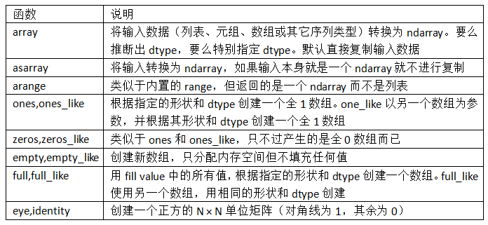
二、创建ndarray数组

ndarray：N维数组对象（矩阵），所有元素必须是相同类型。 
ndarray属性：ndim属性，表示维度个数；shape属性，表示各维度大小；dtype属性，表示数据类型。

# -*- coding: utf-8 -*-

import numpy

print '使用列表生成一维数组'
data = [1,2,3,4]
x = numpy.array(data)
print data #列表 [1, 2, 3, 4]
print x #打印数组 [1 2 3 4]
print x.size #打印元数的个数 4
print x.shape #打印数组各个维度的长度 (4,)
print x.dtype #打印数组元素的类型 int64

print '使用列表生成二维数组'
data = [[1,2],[3,4],[5,6]]
x = numpy.array(data)
print x #打印数组 [[1 2][3 4][5 6]]
print x.ndim #打印数组的维度 2
print x.shape #打印数组各个维度的长度。shape是一个元组 (3,2)

print '使用zero/ones/empty创建数组:根据shape来创建'
x = numpy.zeros(6) #创建一维长度为6的，元素都是0一维数组
print x
x = numpy.zeros((2,3)) #创建一维长度为2，二维长度为3的二维0数组
print x
x = numpy.ones((2,3)) #创建一维长度为2，二维长度为3的二维1数组
print x
x = numpy.empty((3,3)) #创建一维长度为2，二维长度为3,未初始化的二维数组
print x

print '使用arrange生成连续元素'
print numpy.arange(6) # [0,1,2,3,4,5,] 开区间
print numpy.arange(0,6,2)  # [0, 2，4]

print '使用random生成随机数组：均匀分布'
x = x.random.random((2, 3)) #创建指定形状的数组(范围在0至1之间)
print x
x = np.random.rand(10, 10)#创建指定形状(示例为10行10列)的数组(范围在0至1之间， 均匀分布)
print x
x = np.random.randn(10, 10)#创建指定形状(示例为10行10列)的数组(标准正态分布)
print x
x = np.random.uniform(0, 100)#创建指定范围内的一个数
print x
x = np.random.randint(0, 100, 6).reshape(3, 2) #创建指定范围内的一个整数数组，3×2的数组
print x
x = np.random.randint(0, 100, size=(4, 4)) #创建指定范围内的一个整数数组，4×4的数组
print x

print '使用random生成随机数组：正态分布'
x = np.random.normal(0, 0.01, (3, 4))#均值为0，方差为0.01，3×4的数组
print x

三、ndarray的矢量化计算

矢量运算：相同大小的数组键间的运算应用在元素上 
矢量和标量运算：“广播”— 将标量“广播”到各个元素

print 'ndarray数组与标量/数组的运算'
x = numpy.array([1,2,3]) 
print x*2 # [2 4 6]
print x>2 # [False False  True]
print x == 2 #[False True False]
equal_to_two = (x == 2)
print x[equal_to_two] #[2]
y = numpy.array([3,4,5])
print x+y # [4 6 8]
print x>y # [False False False]

四、ndarray数组的基本索引和切片

一维数组的索引：与Python的列表索引功能相似

多维数组的索引：

• arr[r1:r2, c1:c2]
• arr[1,1] 等价 arr[1][1]
• [:] 代表某个维度的数据

print 'ndarray的基本索引'
x = numpy.array([[1,2],[3,4],[5,6]])
print x[0] # [1,2]
print x[0][1] # 2,普通python数组的索引
print x[0,1] # 同x[0][1]，ndarray数组的索引
x = numpy.array([[[1, 2], [3,4]], [[5, 6], [7,8]]])
print x[0] # [[1 2],[3 4]]
y = x[0].copy() # 生成一个副本
z = x[0] # 未生成一个副本
print y #  [[1 2],[3 4]]
print y[0,0] # 1
y[0,0] = 0 
z[0,0] = -1
print y # [[0 2],[3 4]]
print x[0] # [[-1 2],[3 4]]
print z # [[-1 2],[3 4]]

print 'ndarray的切片'
x = numpy.array([1,2,3,4,5])
print x[1:3] # [2,3] 右边开区间
print x[:3] # [1,2,3] 左边默认为 0
print x[1:] # [2,3,4,5] 右边默认为元素个数
print x[0:4:2] # [1,3] 下标递增2
x = numpy.array([[1,2],[3,4],[5,6]])
print x[:2] # [[1 2],[3 4]]
print x[:2,:1] # [[1],[3]]
x[:2,:1] = 0 # 用标量赋值
print x # [[0,2],[0,4],[5,6]]
x[:2,:1] = [[8],[6]] # 用数组赋值
print x # [[8,2],[6,4],[5,6]]

五、ndarray数组的布尔索引和花式索引 

布尔索引：使用布尔数组作为索引。arr[condition]，condition为一个条件/多个条件组成的布尔数组。

print 'ndarray的布尔型索引'
x = numpy.array([3,2,3,1,3,0])
# 布尔型数组的长度必须跟被索引的轴长度一致
y = numpy.array([True,False,True,False,True,False]) 
print x[y] # [3,3,3] 
print x[y==False] # [2,1,0]
print x>=3 # [ True False  True False  True  False]
print x[~(x>=3)] # [2,1,0]
print (x==2)|(x==1) # [False  True False  True False False]
print x[(x==2)|(x==1)] # [2 1]
x[(x==2)|(x==1)] = 0
print x # [3 0 3 0 3 0]

花式索引：使用整型数组作为索引。

print 'ndarray的花式索引:使用整型数组作为索引'
x = numpy.array([1,2,3,4,5,6])
print x[[0,1,2]] # [1 2 3]
print x[[-1,-2,-3]] # [6,5,4]
x = numpy.array([[1,2],[3,4],[5,6]])
print x[[0,1]] # [[1,2],[3,4]]
print x[[0,1],[0,1]] # [1,4] 打印x[0][0]和x[1][1]
print x[[0,1]][:,[0,1]] # 打印01行的01列 [[1,2],[3,4]]
# 使用numpy.ix_()函数增强可读性
print x[numpy.ix_([0,1],[0,1])] #同上 打印01行的01列 [[1,2],[3,4]]
x[[0,1],[0,1]] = [0,0]
print x # [[0,2],[3,0],[5,6]]

六、ndarray数组的转置和轴对换

数组的转置/轴对换只会返回源数据的一个视图，不会对源数据进行修改。

print 'ndarray数组的转置和轴对换'
k = numpy.arange(9) #[0,1,....8]
m = k.reshape((3,3)) # 改变数组的shape复制生成2维的，每个维度长度为3的数组
print k # [0 1 2 3 4 5 6 7 8]
print m # [[0 1 2] [3 4 5] [6 7 8]]
# 转置(矩阵)数组：T属性 : mT[x][y] = m[y][x]
print m.T # [[0 3 6] [1 4 7] [2 5 8]]
# 计算矩阵的内积 xTx
print numpy.dot(m,m.T) # numpy.dot点乘
# 高维数组的轴对象
k = numpy.arange(8).reshape(2,2,2)
print k # [[[0 1],[2 3]],[[4 5],[6 7]]]
print k[1][0][0]
# 轴变换 transpose 参数:由轴编号组成的元组
m = k.transpose((1,0,2)) # m[y][x][z] = k[x][y][z]
print m # [[[0 1],[4 5]],[[2 3],[6 7]]]
print m[0][1][0]
# 轴交换 swapaxes (axes：轴)，参数:一对轴编号
m = k.swapaxes(0,1) # 将第一个轴和第二个轴交换 m[y][x][z] = k[x][y][z]
print m # [[[0 1],[4 5]],[[2 3],[6 7]]]
print m[0][1][0]
# 使用轴交换进行数组矩阵转置
m = numpy.arange(9).reshape((3,3))
print m # [[0 1 2] [3 4 5] [6 7 8]]
print m.swapaxes(1,0) # [[0 3 6] [1 4 7] [2 5 8]]

七、ndarray通用函数

通用函数（ufunc）是一种对ndarray中的数据执行元素级运算的函数。

通用函数（即ufunc）是一种对ndarray中的数据执行元素级运算的函数。你可以将其看做简单函数（接受一个或多个标量值，并产生一个或多个标量值）的矢量化包装器。

print '一元ufunc示例'
x = numpy.arange(6)
print x # [0 1 2 3 4 5]
print numpy.square(x) # [ 0  1  4  9 16 25]
x = numpy.array([1.5,1.6,1.7,1.8])
y,z = numpy.modf(x)
print y # [ 0.5  0.6  0.7  0.8]
print z # [ 1.  1.  1.  1.]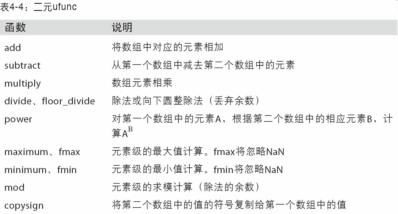

 

print '二元ufunc示例'
x = numpy.array([[1,4],[6,7]])
y = numpy.array([[2,3],[5,8]])
print numpy.maximum(x,y) # [[2,4],[6,8]]
print numpy.minimum(x,y) # [[1,3],[5,7]]
A = np.array([[1,1],[0,1]])
B = np.array([[2,0],[3,4]])
print A
print B
print A*B #对应元素相乘[[2 0][0 4]]
print np.multiply(A,B)#对应元素相乘[[2 0][0 4]]
print A.dot(B) #矩阵乘法[[5 4][3 4]]
print np.dot(A,B)#矩阵乘法[[5 4][3 4]]

八、利用数组进行数据处理

NumPy数组使你可以将许多种数据处理任务表述为简洁的数组表达式（否则需要编写循环）。用数组表达式代替循环的做法，通常被称为矢量化。一般来说，矢量化数组运算要比等价的纯Python方式快上一两个数量级（甚至更多），尤其是各种数值计算。

# -*- coding: utf-8 -*-
print '计算函数sqrt(x^2+y^2)'

points = np.arange(-5, 5, 0.01) # 1000 equally spaced points
xs, ys = np.meshgrid(points, points)#np.meshgrid函数接受两个一维数组，并产生两个二维矩阵
z = np.sqrt(xs ** 2 + ys ** 2)
print z
'''
[[ 7.0711,  7.064 ,  7.0569, ...,  7.0499,  7.0569,  7.064 ],
       [ 7.064 ,  7.0569,  7.0499, ...,  7.0428,  7.0499,  7.0569],
       [ 7.0569,  7.0499,  7.0428, ...,  7.0357,  7.0428, 7.0499],
       ..., 
       [ 7.0499,  7.0428,  7.0357, ...,  7.0286,  7.0357,  7.0428],
       [ 7.0569,  7.0499,  7.0428, ...,  7.0357,  7.0428,  7.0499],
       [ 7.064 ,  7.0569,  7.0499, ...,  7.0428,  7.0499,  7.0569]]

'''

将条件逻辑表述为数组运算:numpy.where函数是三元表达式x if condition else y的矢量化版本。np.where(condition, x, y)，第一个参数为一个布尔数组，第二个参数和第三个参数可以是标量也可以是数组。

print 'where函数的使用'
cond = numpy.array([True,False,True,False])
x = numpy.where(cond,-2,2)
print x # [-2  2 -2  2]
cond = numpy.array([1,2,3,4])
x = numpy.where(cond>2,-2,2)
print x # [ 2  2 -2 -2]
y1 = numpy.array([-1,-2,-3,-4])
y2 = numpy.array([1,2,3,4])
x = numpy.where(cond>2,y1,y2) # 长度须匹配
print x # [1,2,-3,-4]

print 'where函数的嵌套使用'
y1 = numpy.array([-1,-2,-3,-4,-5,-6])
y2 = numpy.array([1,2,3,4,5,6])
y3 = numpy.zeros(6)
cond = numpy.array([1,2,3,4,5,6])
x = numpy.where(cond>5,y3,numpy.where(cond>2,y1,y2))
print x # [ 1.  2. -3. -4. -5.  0.]

九、ndarray常用的统计方法

print 'numpy的基本统计方法'
x = numpy.array([[1,2],[3,3],[1,2]]) #同一维度上的数组长度须一致
print x.mean() # 2
print x.mean(axis=1) # 对每一行的元素求平均
print x.mean(axis=0) # 对每一列的元素求平均
print x.sum() #同理 12
print x.sum(axis=1) # [3 6 3]
print x.max() # 3
print x.max(axis=1) # [2 3 2]
print x.cumsum() # [ 1  3  6  9 10 12]
print x.cumprod() # [ 1  2  6 18 18 36]

这些方法中，布尔值会被强制转换为1（True）和0（False）。用于布尔数组的统计方法：

• sum : 统计数组/数组某一维度中的True的个数
• any： 统计数组/数组某一维度中是否存在一个/多个True
• all：统计数组/数组某一维度中是否都是True

print '用于布尔数组的统计方法'
x = numpy.array([[True,False],[True,False]])
print x.sum() # 2
print x.sum(axis=1) # [1,1]
print x.any(axis=0) # [True,False]
print x.all(axis=1) # [False,False]

 

十、ndarray数组的去重以及集合运算

print 'ndarray的唯一化和集合运算'
x = numpy.array([[1,6,2],[6,1,3],[1,5,2]])
print numpy.unique(x) # [1,2,3,5,6]
y = numpy.array([1,6,5])
print numpy.in1d(x,y) # [ True  True False  True  True False  True  True False]
print numpy.setdiff1d(x,y) # [2 3]
print numpy.intersect1d(x,y) # [1 5 6]

十一、用于数组的文件输入输出

NumPy能够读写磁盘上的文本数据或二进制数据。np.save和np.load是读写磁盘数组数据的两个主要函数。默认情况下，数组是以未压缩的原始二进制格式保存在扩展名为.npy的文件。如果文件路径末尾没有扩展名.npy，则该扩展名会被自动加上。

arr = np.arange(10)
np.save('some_array', arr)
np.load('some_array.npy')#array([0, 1, 2, 3, 4, 5, 6, 7, 8, 9])
np.savez('array_archive.npz', a=arr, b=arr)#通过np.savez可以将多个数组保存到一个未压缩文件中
arch = np.load('array_archive.npz')
print arch['b']  #加载.npz文件时，你会得到一个类似字典的对象
#如果要将数据压缩，可以使用numpy.savez_compressed
np.savez_compressed('arrays_compressed.npz', a=arr, b=arr)

十二、numpy中的线性代数

线性代数（如矩阵乘法、矩阵分解、行列式以及其他方阵数学等）是任何数组库的重要组成部分。

import numpy.linalg 模块。线性代数（linear algebra）

print '线性代数'
import numpy.linalg as nla
print '矩阵点乘'
x = numpy.array([[1,2],[3,4]])
y = numpy.array([[1,3],[2,4]])
print x.dot(y) # [[ 5 11][11 25]]
print numpy.dot(x,y) # # [[ 5 11][11 25]]
print '矩阵求逆'
x = numpy.array([[1,1],[1,2]])
y = nla.inv(x) # 矩阵求逆（若矩阵的逆存在）
print x.dot(y) # 单位矩阵 [[ 1.  0.][ 0.  1.]]
print nla.det(x) # 求行列式
q,r = nla.qr(x) #QR分解
print q
print r

十三、伪随机数生成

numpy.random模块对Python内置的random进行了补充，增加了一些用于高效生成多种概率分布的样本值的函数。

x= np.random.rand(3,3)
print x  #产生均匀分布的样本值
x = np.random.randint(0,10).reshape(3,2)
print x  #产生0～10随机整数组成的矩阵
x = np.random.randn(3,3)
print x #产生正态分布（均值为0，标准差为1）的样本值，矩阵为3×3

 十四、ndarray对象的内部机理

NumPy的ndarray提供了一种将同质数据块（可以是连续或跨越）解释为多维数组对象的方式。正如你之前所看到的那样，数据类型（dtype）决定了数据的解释方式，比如浮点数、整数、布尔值等。

ndarray如此强大的部分原因是所有数组对象都是数据块的一个跨度视图（strided view）。你可能想知道数组视图arr[::2,::-1]不复制任何数据的原因是什么。简单地说，ndarray不只是一块内存和一个dtype，它还有跨度信息，这使得数组能以各种步幅（step size）在内存中移动。更准确地讲，ndarray内部由以下内容组成：

• 一个指向数据（内存或内存映射文件中的一块数据）的指针。
• 数据类型或dtype，描述在数组中的固定大小值的格子。
• 一个表示数组形状（shape）的元组。
• 一个跨度元组（stride），其中的整数指的是为了前进到当前维度下一个元素需要“跨过”的字节数。

                                                                                     Numpy的ndarray对象

十五、ndarray数组重塑 

多数情况下，你可以无需复制任何数据，就将数组从一个形状转换为另一个形状。只需向数组的实例方法reshape传入一个表示新形状的元组即可实现该目的。

print 'ndarray数组重塑'
x = numpy.arange(0,6) #[0 1 2 3 4]
print x #[0 1 2 3 4]
print x.reshape((2,3)) # [[0 1 2][3 4 5]]
print x #[0 1 2 3 4]
print x.reshape((2,3)).reshape((3,2)) # [[0 1][2 3][4 5]]
y = numpy.array([[1,1,1],[1,1,1]])
x = x.reshape(y.shape)
print x # [[0 1 2][3 4 5]]
print x.flatten() # [0 1 2 3 4 5]
x.flatten()[0] = -1 # flatten返回的是拷贝
print x # [[0 1 2][3 4 5]]
print x.ravel() # [0 1 2 3 4 5]
x.ravel()[0] = -1 # ravel返回的是视图（引用） 
print x # [[-1 1 2][3 4 5]]
print "维度大小自动推导"
arr = numpy.arange(15)
print arr.reshape((5, -1)) # 15 / 5 = 3

如果结果中的值与原始数组相同，ravel不会产生源数据的副本。flatten方法的行为类似于ravel，只不过它总是返回数据的副本。

十六、数组的合并和拆分 

print '数组的合并与拆分'
x = numpy.array([[1, 2, 3], [4, 5, 6]])
y = numpy.array([[7, 8, 9], [10, 11, 12]])
print numpy.concatenate([x, y], axis = 0)  
# 竖直组合 [[ 1  2  3][ 4  5  6][ 7  8  9][10 11 12]]
print numpy.concatenate([x, y], axis = 1)  
# 水平组合 [[ 1  2  3  7  8  9][ 4  5  6 10 11 12]]
print '垂直stack与水平stack'
print numpy.vstack((x, y)) # 垂直堆叠:相对于垂直组合
print numpy.hstack((x, y)) # 水平堆叠：相对于水平组合
# dstack：按深度堆叠
print numpy.split(x,2,axis=0) 
# 按行分割 [array([[1, 2, 3]]), array([[4, 5, 6]])]
print numpy.split(x,3,axis=1) 
# 按列分割 [array([[1],[4]]), array([[2],[5]]), array([[3],[6]])]

# 堆叠辅助类
import numpy as np
arr = np.arange(6)
arr1 = arr.reshape((3, 2))
arr2 = np.random.randn(3, 2)
print 'r_用于按行堆叠'
print np.r_[arr1, arr2]
'''
[[ 0.          1.        ]
 [ 2.          3.        ]
 [ 4.          5.        ]
 [ 0.22621904  0.39719794]
 [-1.2201912  -0.23623549]
 [-0.83229114 -0.72678578]]
'''
print 'c_用于按列堆叠'
print np.c_[np.r_[arr1, arr2], arr]
'''
[[ 0.          1.          0.        ]
 [ 2.          3.          1.        ]
 [ 4.          5.          2.        ]
 [ 0.22621904  0.39719794  3.        ]
 [-1.2201912  -0.23623549  4.        ]
 [-0.83229114 -0.72678578  5.        ]]
'''
print '切片直接转为数组'
print np.c_[1:6, -10:-5]
'''
[[  1 -10]
 [  2  -9]
 [  3  -8]
 [  4  -7]
 [  5  -6]]
'''

 十七、元素的重复操作：tile和repeat

对数组进行重复以产生更大数组的工具主要是repeat和tile这两个函数。repeat会将数组中的各个元素重复一定次数，从而产生一个更大的数组。tile的功能是沿指定轴向堆叠数组的副本。

print '数组的元素重复操作'
x = numpy.array([[1,2],[3,4]])
print x.repeat(2) # 按元素重复 [1 1 2 2 3 3 4 4]
print x.repeat(2,axis=0) # 按行重复 [[1 2][1 2][3 4][3 4]]
print x.repeat(2,axis=1) # 按列重复 [[1 1 2 2][3 3 4 4]]
x = numpy.array([1,2])
print numpy.tile(x,2) # tile瓦片：[1 2 1 2]
print numpy.tile(x, (2, 2))  # 指定从低维到高维依次复制的次数。 
# [[1 2 1 2][1 2 1 2]]

十八、广播

广播（broadcasting）指的是不同形状的数组之间的算术运算的执行方式。

arr = np.random.randn(4, 3)
mean = arr.mean(0) #[-0.3928, -0.3824, -0.8768]
demeaned = arr - arr.mean(0)
print demeaned
'''
[[ 0.3937,  1.7263,  0.1633],
 [-0.4384, -1.9878, -0.9839],
 [-0.468 ,  0.9426, -0.3891],
 [ 0.5126, -0.6811,  1.2097]]
'''
row_mean = arr.mean(1)
print row_mean.shape #(4,)
demeaned = arr - row_mean
print demeaned
#ValueError:operands count not be broadcast together with shape (4,3) (4,)
demeaned = arr - row_mean.reshape(4,1)
print demeaned

                                                                                 一维数组在轴0上的广播 

                                                                                  三维数组在轴0上的广播

 

 于是就有了一个非常普遍的问题（尤其是在通用算法中），即专门为了广播而添加一个长度为1的新轴。虽然reshape是一个办法，但插入轴需要构造一个表示新形状的元组。这是一个很郁闷的过程。NumPy数组提供了一种通过索引机制插入轴的特殊语法。通过特殊的np.newaxis属性以及“全”切片来插入新轴。

arr = np.zeros((4, 4))
arr_3d = arr[:, np.newaxis, :]
print arr_3d.shape #(4,1,4)

#三维广播
arr = np.random.randn(3, 4, 5)
depth_means = arr.mean(2)
print depth_means
'''
[[-0.4735,  0.3971, -0.0228,  0.2001],
 [-0.3521, -0.281 , -0.071 , -0.1586],
 [ 0.6245,  0.6047,  0.4396, -0.2846]]
'''
print depth_means.shape #(3,4)
demeaned = arr - depth_means[:, :, np.newaxis]#(3,4,5) - (3,4,1)
print demeaned.mean(2)
'''
[[ 0.,  0., -0., -0.],
 [ 0.,  0., -0.,  0.],
 [ 0.,  0., -0., -0.]]
'''

通过广播设置数组的值

arr = np.zeros((4, 3))
arr[:] = 5
print arr
'''
[[ 5.,  5.,  5.],
 [ 5.,  5.,  5.],
 [ 5.,  5.,  5.],
 [ 5.,  5.,  5.]]
'''
#想要用一个一维数组来设置目标数组的各列，只要保证形状兼容就可以
col = np.array([1.28, -0.42, 0.44, 1.6])
arr[:] = col[:, np.newaxis]
print arr
'''
[[ 1.28,  1.28,  1.28],
 [-0.42, -0.42, -0.42],
 [ 0.44,  0.44,  0.44],
 [ 1.6 ,  1.6 ,  1.6 ]]
'''
arr[:2] = [[-1.37], [0.509]]
print arr
'''
[[-1.37 , -1.37 , -1.37 ],
 [ 0.509,  0.509,  0.509],
 [ 0.44 ,  0.44 ,  0.44 ],
 [ 1.6  ,  1.6  ,  1.6  ]]
'''

十九、排序

使用sort对数组/数组某一维度进行就地排序（会修改数组本身）。

print '.sort的就地排序'
x = numpy.array([[1,6,2],[6,1,3],[1,5,2]])
x.sort(axis=1) 
print x # [[1 2 6] [1 3 6] [1 2 5]]


x = np.array([1, 2, 6, 4])
print x #[1 2 6 4]
x.sort() 
print x #[1 2 4 6]

x = np.array([1, 2, 6, 4])
print x #[1 2 6 4]
y = np.sort(x)  #非就地排序：numpy.sort()可产生数组的副本
print x #[1 2 6 4]
print y #[1 2 4 6]
print x[::-1] #[4 6 2 1] #反序

你可能注意到了，这两个排序方法都不可以被设置为降序。其实这也无所谓，因为数组切片会产生视图（也就是说，不会产生副本，也不需要任何其他的计算工作）。许多Python用户都很熟悉一个有关列表的小技巧：values[::-1]可以返回一个反序的列表。对ndarray也是如此。

arr = np.random.randn(3, 5)
print arr
'''
[[ 0.5955, -0.2682,  1.3389, -0.1872,  0.9111],
       [-0.3215,  1.0054, -0.5168,  1.1925, -0.1989],
       [ 0.3969, -1.7638,  0.6071, -0.2222, -0.2171]]

'''
arr.sort(axis=1)
print arr
'''
[[-0.2682, -0.1872,  0.5955,  0.9111,  1.3389],
       [-0.5168, -0.3215, -0.1989,  1.0054,  1.1925],
       [-1.7638, -0.2222, -0.2171,  0.3969,  0.6071]]

'''
print arr[:, ::-1] #反序数组，注意有 维度-1 个‘：，’符号
'''
[[ 1.3389,  0.9111,  0.5955, -0.1872, -0.2682],
       [ 1.1925,  1.0054, -0.1989, -0.3215, -0.5168],
       [ 0.6071,  0.3969, -0.2171, -0.2222, -1.7638]]
'''

间接排序：argsort和lexsort

values = np.array([5, 0, 1, 3, 2])
indexer = values.argsort()
priint indexer #[1, 2, 4, 3, 0]
print values[indexer] #[0, 1, 2, 3, 5]

#lexsort跟argsort差不多，只不过它可以一次性对多个键数组执行间接排序（字典序）。
first_name = np.array(['Bob', 'Jane', 'Steve', 'Bill', 'Barbara'])
last_name = np.array(['Jones', 'Arnold', 'Arnold', 'Jones', 'Walters'])
sorter = np.lexsort((first_name, last_name))
print sorter #[1, 2, 3, 0, 4]

二十、性能建议

使用NumPy的代码的性能一般都很不错，因为数组运算一般都比纯Python循环快得多。下面大致列出了一些需要注意的事项：

• 将Python循环和条件逻辑转换为数组运算和布尔数组运算。
• 尽量使用广播。
• 避免复制数据，尽量使用数组视图（即切片）。
• 利用ufunc及其各种方法。

总结：

本文主要参考《利用Python进行数据分析·第2版》和博客https://blog.csdn.net/cxmscb/article/details/54583415完成编写。