AdaLoGN Adaptive Logic Graph Network for Reasoning-Based Machine Reading 论文及代码解读

论文介绍

论文题目：AdaLoGN Adaptive Logic Graph Network for Reasoning-Based Machine Reading Comprehension
会议：ACL 2022
论文链接：https://aclanthology.org/2022.acl-long.494/
代码地址： https://github.com/nju-websoft/AdaLoGN.
作者：Xiao Li and Gong Cheng and Ziheng Chen and Yawei Sun and Yuzhong Qu
机构：State Key Laboratory for Novel Software Technology, Nanjing University, Nanjing, China

摘要：近期的机器阅读理解数据集(如ReClor和LogiQA)要求模型能够对文本执行逻辑推理。传统的神经网络模型难以实现逻辑推理，而符号推理不能直接应用于文本。为了应对这一挑战，提出了一种神经-符号方法，该方法通过表示文本单元之间逻辑关系的图来传递消息，以预测答案。它结合了一个自适应逻辑图网络(AdaLoGN)，自适应地推断逻辑关系来扩展图，本质上实现了神经推理和符号推理之间的相互和迭代强化。我们还实现了一种新的子图到节点的消息传递机制，以增强回答多项选择题的上下文选项交互。该方法在ReClor和LogiQA上取得了较好的结果。

论文内容

简介

机器阅读理解(MRC)已经引起了广泛的研究关注。早期的MRC数据集对于最先进的神经网络方法来说并不困难。事实上，BERT (Devlin等人，2019)在SQuAD上的表现优于人类(Rajpurkar等人，2016)。最近的数据集变得更具挑战性。例如，ReClor (Y u et al, 2020)和LogiQA (Liu et al, 2020)需要对文本中描述的逻辑关系进行理解和推理，其中神经网络方法表现出不令人满意的性能。

例如，下图中的MRC任务。Context由一组描述基本语篇单元(elementary discourse units, edu)之间逻辑关系的语篇命题组成(Mann和Thompson, 1988)。例如，第一句话描述了两个edu之间的含义:“公司获得项目A (the company gets project A) ”意味着“产品B可以按时投放市场 (product B can be put on the market on schedule) ”。在命题演算的帮助下，人类可以将命题形式化，然后应用命题逻辑中的推理规则来证明选项C中的命题。然而，机器如何解决这样的任务呢?

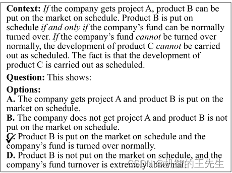
图 1：一个MRC任务示例(改编自LogiQA中的一组数据)。逻辑连接词用斜体突出显示。√标记正确答案。

为了解决这个问题，传统的神经模型不足以提供所需的推理能力，而符号推理器不能直接应用于非结构化文本。一个具有价值的研究方向是考虑神经符号解决方案，例如最近的DAGN方法(Huang et al, 2021a)。它将上下文和每个选项分解为一组edu，并将它们与话语关系连接成图表。然后执行基于图神经网络(GNN)的推理来预测答案。

现有方法及局限性：

1. 尽管有图的表示，但它主要是一种关于语篇关系的神经方法。对逻辑关系（如暗示、否定）所需的符号推理是否可以适当地近似，是值得商榷的。
   Despite the graph representation, it is predominantly a neural method over discourse relations. It is debatable whether the required symbolic reasoning over logical relations (e.g., implication, negation) can be properly approximated. （对于这一点，作者将语篇关系转换为逻辑关系，并增加了自适应推理策略）
2. 构造出来的图通常是比较松散的，且多为长路径组成。在现有GNN模型中实现的节点间消息传递策略中，无法提供足够的上下文和选项之间的交互作用，这对于回答多项选择题至关重要。
   The graph is often loosely connected and composed of long paths. Node-to-node message passing implemented in existing GNN models (Kipf and Welling, 2017; Schlichtkrull et al, 2018; V elickovic et al, 2018) is prone to provide insufficient interaction between the context and the option, which is critical to answering a multiple-choice question. （对于这一点，作者使用了子图到节点的消息传递机制）

• 语篇关系：可参考https://www.jianshu.com/p/061bc50ca21c或论文《Easily identifiable discourse relations》

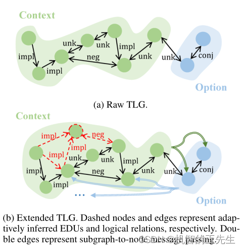
图2：本文所提出的TLG图的例子

本文的方法：
本文的方法遵循DAGN的基本框架，即首先构造图，然后做基于图的推理。但本文采用了一种新的神经-符号方法来克服两个局限性。具体如下：

• 为了解决第一个限制问题，构建一个文本逻辑图(text logic graph, TLG)，表示edu及其逻辑关系，而不是语篇关系，因此可以显式地执行符号推理，以推断出逻辑关系来扩展TLG，如图2所示。推断出的关系可以为后续基于图的消息传递提供关键的连接（后文介绍了三个扩展规则），即符号推理加强了神经推理。虽然琐碎地计算和接纳演绎闭包可能会用不相关的连接来扩展TLG，从而误导信息传递，但利用神经推理的信号来适应性地接纳相关的扩展，也就是神经推理加强了符号推理（后文介绍了相关性分数计算）。同时，通过在每次迭代中用上一次迭代的信号重新启动推理来迭代上述的相互强化，以适应推理过程的修正，并允许神经-符号的充分互动。
• 为了解决第二个限制问题，在TLG的上下文子图中聚合信息，并采用一种新的子图到节点的消息传递机制来增强整体上下文的交互。

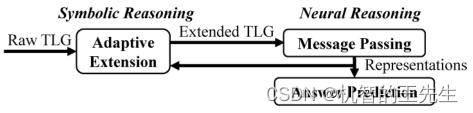
图3：主要观点：符号推理和神经推理之间的相互迭代强化

本文贡献：

1. 一种新颖的神经符号方法，其中神经和符号推理相互并迭代地相互加强；
2. 基于图的神经推理中基于聚合的消息传递增强。

方法

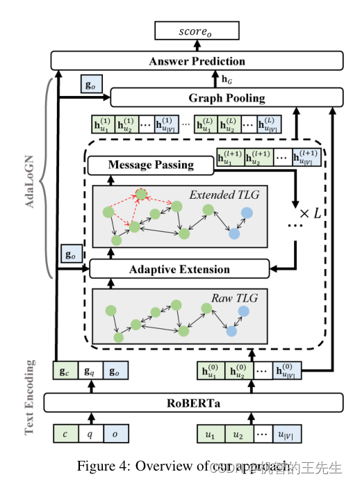
图4： AdaLoGN模型结构图

首先介绍定义部分：MRC任务由一个上下文$c$，一个问题$q$和一组选项$O$组成。在$O$中只有一个选项是给定$c$和$q$的正确答案。任务的目标是找到这个选项。

本文提出的AdaLoGN模型结构图如上图所示。对于每个选项$o\in O$，通过预训练的语言模型生成$c,q,o$的表示(即$g_c,g_q,g_o$)，构造一个原始的TLG，其中节点(即$u_1，\dots ，u_{|V|}$)表示从$c,q,o$中提取的edu，边表示它们的逻辑关系。用它们的初始表示(即$h_{u_1}^{(0)}，\dots \dots ，h_{u_{|V|}}^{(0)}$)，以迭代的方式自适应扩展TLG(即符号推理)，然后传递消息(即神经推理)以更新节点表示(即$h_{u_1}^{(l+1)}，\dots ，h_{u_{|V|}}^{(l+1)}$)用于生成TLG的表示(即$h_G$)。最后，基于上述表示预测$o$(即$scor{e}_o$)的正确性。

文本编码器

使用RoBERTa预训练语言模型作为文本编码器，得到：$[g_{<s>};g_{c_1};...g_{</s>};g_{q_1};...;g_{o_1};g_{</s>}]=RoBERTa(<s>c_1...</s>q_1...o_1...,</s>)$
对输出向量求平均，得到$c,q,o$的表示：
${\mathbf{g}}_c=\frac{1}{|c|}{\sum }_{i=1}^{|c|}{\mathbf{g}}_{c_i},{\mathbf{g}}_q=\frac{1}{|q|}{\sum }_{i=1}^{|q|}{\mathbf{g}}_{q_i},{\mathbf{g}}_o=\frac{1}{|o|}{\sum }_{i=1}^{|o|}{\mathbf{g}}_{o_i}$
对应代码（RobertaAdaLoGN.py文件中的_get_split_origin_context_answer_representation）：

context_origin_representations = [torch.mean(last_hidden_states[index, si[0][0]:si[0][1], :], dim=0).view(self.config.hidden_size) for index, si in enumerate(sep_interval)]
question_origin_representations = [torch.mean(last_hidden_states[index, si[1][0]:si[1][1], :], dim=0) for index, si in enumerate(sep_interval)]
answer_origin_representations = [torch.mean(last_hidden_states[index, si[2][0]:si[2][1], :], dim=0) for index, si in enumerate(sep_interval)]

文本逻辑图-TLG

对于文本部分，除了编码之外，还根据文本进行TLG图构建。构建方法如下：

TLG图定义

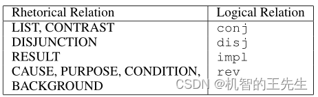
对于一段文本，它的TLG图是一个有向图$G=<V,E>$，其中，$V$是所有的EDU节点集合，$E\subseteq V\times R\times V$是一组带有标记（逻辑关系）的有向边。本文仅考虑六种逻辑关系： R = { R=\{ R={ conj, disj, impl, neg, rev, unk $\}$

• conjunction ($conj$), disjunction ($disj$), implication ($impl$), and negation ($neg$)是命题逻辑中标准的逻辑连接词；
• 引入implication ($rev$) 来表示$impl$的逆关系；
• $unk$表示未知关系。
  由于$conj,disj,neg,unk$是对称关系，因此用它们标记的边是双向的。语篇关系与逻辑关系的映射如下表所示。

表1：语篇关系与逻辑关系对照表

这部分处理代码对应文件data_utils_preprocess.py文件中的construct_relation_graph_new函数

        for hash_id in edus:
            for linked_edu in edus[hash_id]['linkedContexts']:
                target_id = linked_edu['targetID']
                relation = linked_edu['relation']

                if target_id == 'deleted':
                    continue
                if relation in ['UNKNOWN_SUBORDINATION', 'ATTRIBUTION', 'SPATIAL']:
                    continue
                elif relation in ['BACKGROUND', 'CAUSE', 'CONDITION', 'PURPOSE', 'CAUSE_C']:
                ...

构造TLG图

首先，采用与Huang等人一致的方法（DAGN）根据$c$和$o$构造初始化的EDUs图。本文采用Graphene工具提取。

还定义了少量的语法规则来识别相互否定的edu，并将它们与自己的否定edu连接起来。这些规则基于part-of-speech tags和dependencies。例如，一个规则检查两个edu之间是否只存在一个副词的反义词。此外，对于文本中相邻的每一对EDU(包括$c$的最后一个EDU和$o$的第一个EDU)均进行连接，如果没有上述逻辑关系，则用$unk$来连接它们。

自适应逻辑图网络 (Adaptive Logic Graph Network, AdaLoGN)

由于TLG由逻辑关系组成，可以应用推理规则明确地进行符号推理，用推断的逻辑关系扩展TLG，以利于后续的神经推理。然而，本文利用神经推理的信号来识别和接纳相关的扩展，而不是计算演绎闭包，因为它可能会提供许多与回答问题无关的关系，并误导神经推理，从而进行自适应扩展。（根据相关性分数和阈值控制是否保留扩展结果）

对于神经推理，执行消息传递来更新节点表征，最后将其汇集到TLG的表征中，用于后续的答案预测。通过在每次迭代中用上一次迭代的信号重新启动对原始TLG的推理来迭代上述过程，以适应推理过程的修正，并让符号推理和神经推理充分地相互作用。

图扩展规则

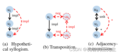
图5 三个推理规则用于图扩展

通俗理解：
（代码位置为：data_utils_preprocess.py的def construct_relation_graph_extension）

• Hypothetical Syllogism： a–impl–>b 且 b–impl–>c 则 a–impl–>c 对应以下代码块：

        for _ in range(max_extension_depth - 1):
            if len(trans_exten_edge_ids[i]) > Config.extension_padding_len:
                break
            for relation_index in range(len(relations[i])):
                if relations[i][relation_index] == imp_relation_id:
                    edge_a, edge_b = graphs[i].edges()[0].numpy().tolist()[relation_index], \
                                     graphs[i].edges()[1].numpy().tolist()[relation_index]
                    for edge_index in range(len(graphs[i].edges()[0].numpy().tolist())):
                        # a--(imp)->b   b--(imp)->c  trans_exten_edge_ids记录 [a,c,imp]  Hypothetical syllogism.
                        if graphs[i].edges()[0].numpy().tolist()[edge_index] == edge_b and (
                                relations[i][edge_index] == imp_relation_id):
                            trans_exten_edge_ids[i].append(
                                [edge_a, graphs[i].edges()[1].numpy().tolist()[edge_index], imp_relation_id])
            edges_a, edges_b = graphs[i].edges()[0].numpy().tolist(), graphs[i].edges()[1].numpy().tolist()
            for index in range(len(trans_exten_edge_ids[i])):
                tmp_edges_id.append(len(edges_a))
                edges_a.append(trans_exten_edge_ids[i][index][0])
                edges_b.append(trans_exten_edge_ids[i][index][1])
                relations[i].append(trans_exten_edge_ids[i][index][2])
            graphs[i] = dgl.graph((edges_a, edges_b))
            assert is_dgl_graph_connected(graphs[i])

• Transposition： a–>impl–>b 且 a–neg–>not_a 且 b–neg–>not_b 则 not_b–impl–>not_a 对应代码块：

        for relation_index in range(len(relations[i])):
            if len(cont_exten_node_ids[i]) + len(trans_exten_edge_ids[i]) > Config.extension_padding_len:
                break
            if relations[i][relation_index] == imp_relation_id:
                edge_a, edge_b = graphs[i].edges()[0].numpy().tolist()[relation_index], \
                                 graphs[i].edges()[1].numpy().tolist()[relation_index]
                sentence_a = (node_sentences_a[i] + node_sentences_b[i])[edge_a].replace('_c', '').replace('_d', '')
                sentence_b = (node_sentences_a[i] + node_sentences_b[i])[edge_b].replace('_c', '').replace('_d', '')

                sentence_a_neg = get_from_new_not_sentence_map(sentence_a)
                sentence_b_neg = get_from_new_not_sentence_map(sentence_b)

                if len(sentence_a_neg) == 0 or len(sentence_b_neg) == 0 or sentence_a_neg[0] == 'None' or \
                        sentence_b_neg[
                            0] == 'None' or 'error when convert' in sentence_a_neg or 'error when convert' in sentence_b_neg:
                    continue
                not_a_node_id = add_node(sentence_a_neg[0] + ('_c' if edge_a < len(node_sentences_a[i]) else '_d'), i,
                                         'c' if edge_a < len(node_sentences_a[i]) else 'd')
                not_b_node_id = add_node(sentence_b_neg[0] + ('_c' if edge_b < len(node_sentences_a[i]) else '_d'), i,
                                         'c' if edge_b < len(node_sentences_a[i]) else 'd')

                add_edge(edge_a, not_a_node_id, 'NOT', i)
                add_edge(not_a_node_id, edge_a, 'NOT', i)
                add_edge(edge_b, not_b_node_id, 'NOT', i)
                add_edge(not_b_node_id, edge_b, 'NOT', i)
                add_edge(not_b_node_id, not_a_node_id, 'IMP', i)
                add_edge(not_a_node_id, not_b_node_id, 'IMP_REV', i)
                cont_exten_node_ids[i].append([edge_a, not_a_node_id, edge_b, not_b_node_id])

• Adjacency-Transmission： a<–unk–>b 且 b–>(con/disj/impl)–>c 则 a–(con/disj/impl)–>c 对应以下代码块：

        for _ in range(max_extension_depth - 1):
            if len(trans_exten_edge_ids[i]) > Config.extension_padding_len:
                break
            for relation_index in range(len(relations[i])):
                if relations[i][relation_index] == imp_relation_id:
                    edge_a, edge_b = graphs[i].edges()[0].numpy().tolist()[relation_index], \
                                     graphs[i].edges()[1].numpy().tolist()[relation_index]
                    for edge_index in range(len(graphs[i].edges()[0].numpy().tolist())):
                        if graphs[i].edges()[0].numpy().tolist()[edge_index] == edge_b and (
                                relations[i][edge_index] == imp_relation_id):
                            trans_exten_edge_ids[i].append(
                                [edge_a, graphs[i].edges()[1].numpy().tolist()[edge_index], imp_relation_id])
            edges_a, edges_b = graphs[i].edges()[0].numpy().tolist(), graphs[i].edges()[1].numpy().tolist()
            for index in range(len(trans_exten_edge_ids[i])):
                tmp_edges_id.append(len(edges_a))
                edges_a.append(trans_exten_edge_ids[i][index][0])
                edges_b.append(trans_exten_edge_ids[i][index][1])
                relations[i].append(trans_exten_edge_ids[i][index][2])
            graphs[i] = dgl.graph((edges_a, edges_b))
            assert is_dgl_graph_connected(graphs[i])

TLG的自适应扩展

依靠来自神经推理的信号来决定哪些推理步骤与回答问题相关，相关的扩展保留。计算方法：对于每个候选$ϵ$，及节点$V_{ϵ}\subset V$，取他们的平均向量作为$ϵ$的表示：
${\mathbf{h}}_{ϵ}=\frac{1}{|V_{ϵ}|}{\sum }_{u_i\in V_{ϵ}}{\mathbf{h}}_{u_i}$
对应代码（RobertaAdaLoGN.py文件中的_get_split_representation）：

node_representations = [torch.stack([torch.mean(last_hidden_states[i, s:e, :], dim=0).view(self.config.hidden_size) for (s, e) in node_interval]) for i, node_interval in enumerate(node_intervals)]

由于图扩展$ϵ$的作用是用于预测选项$o$的正确性的，因此，将其与$o$的表示进行拼接，计算相关性分数：
$re{l}_{ϵ}=\mathrm{sigmoid}($ linear $\left({\mathbf{h}}_{ϵ}\Vert {\mathbf{g}}_o\right))$
对应代码GNNs.py的RGATLayer类的forward函数：

pred_value = self.extension_pred_layer(torch.cat([torch.mean(torch.index_select(graphs_list[i].ndata['h'], dim=0, index=eni), dim=0),
torch.mean(torch.index_select(graphs_list[i].ndata['answer'], dim=0, index=eni), dim=0)],dim=-1))
pred_value = torch.sigmoid(pred_value).view(1)

设置阈值$\tau$，若$re{l}_{ϵ}>\tau$，则保留$ϵ$扩展结果。对应代码：

                if pred_value > Config.extension_threshold:
                    exten_edges[0].append(eni[0].view(-1))
                    exten_edges[1].append(eni[1].view(-1))
                    edge_relation_type.append(exten_edges_ids[i][j][2].view(1))

这个过程是可迭代的，即第$(l+1)$次迭代中，使用raw TLG执行符号推理，使用第$l$次的节点表示${\mathbf{h}}_u^{(l)}$重新计算${\mathbf{h}}_{ϵ}$，$h_u^{(0)}$是由预训练语言模型得到。
每个节点的表示是组成该节点的词的表示的平均值：
${\mathbf{h}}_{u_i}^{(0)}=\frac{1}{|u_i|}{\sum }_{j=1}^{|u_i|}{\mathbf{h}}_{u_{i_j}}$。对应代码：

消息传递

为了让TLG中的节点彼此交互并融合它们的信息，我们的神经推理执行基于图的消息传递，在每次迭代中更新节点表示，从$h_{u_i}^{(l)}到h_{u_i}^{(l+1)}$。由于TLG是一个包含多种类型边的异构图，将R-GCN中的节点到节点消息传递机制作为基础。此外，观察到TLG通常是松散连接的，在有限的迭代中，通过长路径容易导致$V_c$和$V_o$之间的相互作用不足，这不能通过简单地增加迭代次数来缓解，因为它会引起其他问题，如过度平滑。为了增强这种对预测$o$的正确性至关重要的交互，我们引入了一种新的subgraph-to-node消息传递机制，将从子图(例如$V_c$)聚合的信息整体传递到节点(例如，每个$u_i\in V_o$)。

具体来说，在不失通用性的前提下，对于每个$u_i\in V_o$，我们通过$V_c$上的节点表示的注意加权和来计算$V_c$的$u_i$参与的聚合表示：
$\begin{array}{rl}{\mathbf{h}}_{V_c,u_i}^{(l)}& =\sum _{u_j\in V_c}{\alpha }_{i,j}{\mathbf{h}}_{u_j}^{(l)},\text{ where }\\ {\alpha }_{i,j}& ={\mathrm{softmax}}_j\left({\left[a_{i,1};\dots ;a_{i,|V_c|}\right]}^{\top }\right)\\ a_{i,j}& =\mathrm{LeakyReLU}\left(\mathrm{linear}\left({\mathbf{h}}_{u_i}^{(l)}\Vert {\mathbf{h}}_{u_j}^{(l)}\right)\right)\end{array}$
设$N^i$ 是节点$i$的邻域（邻居节点集合），设$N_r^i\subseteq N_i$是逻辑关系$r\in R$下的子集。我们通过向$u_i$的邻居和$V_c$传递消息来更新$u_i$的表示：
$\begin{array}{rl}& {\mathbf{h}}_{u_i}^{(l+1)}=\mathrm{ReLU}(\sum _{r\in R}\sum _{u_j\in N_r^i}\frac{{\alpha }_{i,j}}{\left|N_r^i\right|}{\mathbf{W}}_r^{(l)}{\mathbf{h}}_{u_j}^{(l)}+{\mathbf{W}}_0^{(l)}{\mathbf{h}}_{u_i}^{(l)}\\ & +{\beta }_i{\mathbf{W}}_{\text{subgraph }}^{(l)}{\mathbf{h}}_{V_c,u_i}^{(l)}),\text{ where }\\ & {\alpha }_{i,j}={\mathrm{softmax}}_{i\mathrm{dx}\left(a_{i,j}\right)}\left({\left[\dots ;a_{i,j};\dots \right]}^{\top }\right)\text{ for all }{u}_j\in N^i\text{, }\\ & a_{i,j}=\text{ LeakyReLU }\left(\text{ linear }\left({\mathbf{h}}_{u_i}^{(l)}\Vert {\mathbf{h}}_{u_j}^{(l)}\right)\right)\text{, }\\ & {\beta }_i=\mathrm{sigmoid}\left(\text{ linear }\left({\mathbf{h}}_{u_i}^{(l)}\Vert {\mathbf{h}}_{V_c,u_i}^{(l)}\right)\right),\\ & \end{array}$
其中，${\mathbf{W}}_r^{(l)},{\mathbf{W}}_0^{(l)},{\mathbf{W}}_{\text{subgraph }}^{(l)}$是可学习的参数，$idx(a_{i,j})$返回$a_{i,j}$在$|N^i|$维度向量中（${\left[\dots ;a_{i,j};\dots \right]}^{\top }$）的索引值。类似的，对于每个$u_i\in V_c$，计算由$u_i$参与的$V_o$的聚合表示，表示为$h_{V_o,u_i}^{(l)}$并更新$h_{u_i}^{(l+1)}$。

本文与原R-GCN的对应式有两个不同之处。首先，结合子图到节点的消息传递，并通过门控机制(即${\beta }_i$)控制它。其次，对通过注意机制(即${\alpha }_{i,j}$)传递的节点到节点消息进行加权。

Graph polling

在$L$次迭代之后，对于每个节点$u_i\in V$，用残差连接融合其在所有迭代中的表示：
${\mathbf{h}}_{u_i}^{\text{fus }}={\mathbf{h}}_{u_i}^{(0)}+\mathrm{linear}\left({\mathbf{h}}_{u_i}^{(1)}\Vert \cdots \Vert {\mathbf{h}}_{u_i}^{(L)}\right)$
受Huang等人(2021a)的启发，将所有${\mathbf{h}}_{u_i}^{\text{fus }}$输入双向剩余GRU层，以得到节点表示：
$\left[{\mathbf{h}}_{u_1}^{\mathrm{fnl}};\dots ;{\mathbf{h}}_{u_{|V|}}^{\text{fnl }}\right]=\mathrm{Res}-\mathrm{BiGRU}\left(\left[{\mathbf{h}}_{u_1}^{\text{fus }};\dots ;{\mathbf{h}}_{u_{|V|}}^{\text{fus }}\right]\right)$

通过计算一个$o$-attended的加权和来聚合这些节点表示：
$\begin{array}{rl}{\mathbf{h}}_V& =\sum _{u_i\in V}{\alpha }_i{\mathbf{h}}_{u_i}^{\mathrm{fnl}},\text{ where }\\ {\alpha }_i& ={\mathrm{softmax}}_i\left({\left[a_1;\dots ;a_{|V|}\right]}^{\top }\right)\\ a_i& =\mathrm{LeakyReLU}\left(\mathrm{linear}\left({\mathbf{g}}_o\Vert {\mathbf{h}}_{u_i}^{\mathrm{fnl}}\right)\right)\end{array}$

将${\mathbf{h}}_V$和每次迭代的相关性分数串联起来，得到图$G$的表示：
$\begin{array}{rl}{\mathbf{h}}_G& =\left({\mathbf{h}}_V\Vert re{l}_{{\mathcal{E}}^{(1)}}\Vert \cdots \Vert re{l}_{{\mathcal{E}}^{(L)}}\right),\text{ where }\\ re{l}_{{\mathcal{E}}^{(l)}}& =\frac{1}{\left|{\mathcal{E}}^{(l)}\right|}\sum _{ϵ\in {\mathcal{E}}^{(l)}}re{l}_{ϵ},\end{array}$

答案预测

融合$c,q,o$和TLG的表示${\mathbf{h}}_G$来预测$o$的正确性：
score ${}_o=\mathrm{linear}\left(\tanh \left(\mathrm{linear}\left({\mathbf{g}}_c\Vert {\mathbf{g}}_q\Vert {\mathbf{g}}_o\Vert {\mathbf{h}}_G\right)\right)\right)$

损失函数

设$O_{gold}\in O$为正确答案，本文使用label smoothing优化交叉熵损失函数：
$\mathcal{L}=-(1-\gamma )$ score ${}_{o_{\text{gold }}^{\prime }}^{\prime }-\gamma \frac{1}{|O|}{\sum }_{o_i\in O}$ score ${}_{o_i}^{\prime }$
其中，${\mathrm{score}}_{o_i}^{\prime }=\log \frac{\exp \left({\text{ score }}_{o_i}\right)}{{\sum }_{o_j\in O}\exp \left({\text{ score }}_{o_j}\right)}$ $\gamma$ 是一个预定义的平滑因子。

实验

数据集

本文采用的数据集有ReClor和LogiQA。

表2：在ReClor数据及上的对比实验

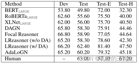
AdaLoGN在测试集上的表现至少优于所有基线方法1.30%。AdaLoGN和LReasoner (w/ DA)均超过60%，与人类水平(63%)相当。

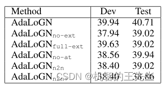
表3：在LogiQA数据及上的对比实验

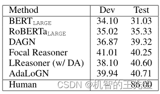
在LogiQA上，如表3所示，AdaLoGN优于测试集上的所有基线方法，包括LReasoner (w/ DA)。尽管如此，结果(40.71%)仍然无法与人类的表现(86%)相提并论。

在ReClor和LogiQA上，AdaLoGN在测试集上超过DAGN 1.39%-1.90%，这证明了该方法在解决第1节中提到的DAGN局限性方面的有效性。

消融实验

表4：消融实验在ReClor数据集上的对比结果

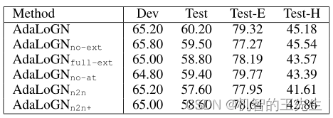
表5：消融实验在LogiQA数据集上的对比结果

其中，no-ext表示不执行图扩展，full-ext表示不进行过滤，no-at表示忽视adjacency-transmission扩展规则，n2n表示仅执行node-to-node的消息传递。n2n+表示Context中的节点与Option中的节点进行连接，边为双向的$unk$。

结果表明：

• 自适应扩展的方法是有效果的，但在神经推理中天真地（naive）注入逻辑推理可能不会产生积极的影响（比no-ext下降还大）
• no-at结果表明，虽然adjacency-transmission扩展规则是启发式规则，但其任然是有用的；
• n2n的结果表明了子图到节点的消息传递是有效的，n2n+结果表明天真地（naive）将图的节点连接在一起可能会产生负面影响。

同时，作者分析了$\tau$的分布，如下图所示：

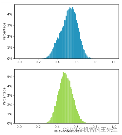
图6： 候选扩展的相关性分数的分布。Top:在Reclor的dev中的结果; Bottom:在LogiQA的dev中的结果

$\tau$的结果呈正态分布，设其为0.6，在ReClor和LogiQA上分别保留了19.57%和4.86%的扩展结果。

误差分析

从每个数据集的开发集中，随机抽取了50个问题，该方法对这些问题输出了错误的答案。作者分析了这些误差的来源。

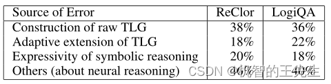
从图中可以看出，主要的错误来自于TLG图的构建不够精确；其次，一些过度的扩展产生了不相关的逻辑关系，可能会误导消息传递；五分之一的错误(18%-20%)是由于符号推理的表达能力有限，即命题逻辑的子集，一些问题需要量词。其他错误可能与神经推理有关，如消息传递或答案预测。

结论

为了应对基于推理的MRC的挑战，文章提出了一种神经-符号方法，其中神经和符号推理通过新的AdaLoGN模型相互迭代地加强。本文还用一种新的子图到节点的消息传递机制来加强基于图的神经推理。由于这些想法是相当普遍的，作者相信它们在MRC之外的各种应用中具有很大的潜力，例如链接预测。

错误分析揭示了该方法的一些缺点。目前仅依靠句法工具从文本中提取一个原始的TLG。未来将探索其他的提取方法以达到更高的质量。还计划应用更多的推理规则并加入量词，以提高符号推理的表达能力。

代码分析

代码地址： https://github.com/nju-websoft/AdaLoGN.

数据预处理

1. 将原始LogiQA数据集的格式(txt)转换为类似ReClor格式的JSON；
2. 使用Graphene工具进行EDUs抽取；

上述步骤可使用作者发布的结果

数据处理

以dev数据集为例
数据处理入口代码在 run_multiple_choice.py 文件中找到

dataset_class = {"LogiGraph": DatasetBertLogiGraph}

...

dev_dataset = (
        dataset_class[data_args.task_name](
            data_dir=data_args.data_dir,
            tokenizer=tokenizer,
            task=data_args.task_name,
            max_seq_length=data_args.max_seq_length,
            overwrite_cache=data_args.overwrite_cache,
            mode=Split.dev_and_test,
        )

具体是在文件data_utils.py中的类DatasetBertLogiGraph中。
首先对文件进行读取，加载为examples，对应代码为：

examples = processor.get_dev_examples(data_dir)

文本文件加载

def get_dev_examples(self, data_dir):
    """See base class."""
    logger.info("LOOKING AT {} dev".format(data_dir))
    return self._create_examples(f'{data_dir}/val.json', "dev")

def _create_examples(self, data_dir, type)

大部分数据在以下代码处获得：
context, endings, graphs, node_sentences_a, node_sentences_b, relations, edge_norms, base_node_ids, cont_exten_node_ids, trans_exten_edge_ids = construct_logic_graph( id_string, return_base_nodes=True)
该部分代码获得的结果包括： context_origin 原始context；endings_origin 原始选项；context 由EDUs组成的Context；endings 由EDUs组成的选项；graphs 由dlg工具生成的图；edge_types 关系边列表；graph_node_nums 记录节点个数；label 答案；nodes_num context和option的节点数总和；exten_nodes_ids 扩展的节点编号；exten_edges_id 扩展的边的编号。

EDUs的加载是在 data_utils_preprocess.py文件中

EDUs = json.load(open(f'{dataset_dir}/{dataset_dir}_EDUs_one.json', 'r', encoding='utf-8'))

TLG图构造及扩展

def construct_logic_graph(id: str, return_base_nodes=False, min_edge_nums=Config.truncate_edges_num)

该函数用于构造文本逻辑图TLG，并执行三个扩展规则。扩展结果存储于trans_exten_edge_ids和cont_exten_node_ids（记录否定关系的）

def construct_relation_graph_extension();

该函数是使用三个扩展规则对图进行扩展的，扩展规则对应代码已贴在上面图扩展规则一节

若图的节点超过了最大节点个数限制，需要执行合并图，函数为construct_relation_graph_merger_nodes

最终加载的数据全部打包在examples中

example = InputExampleBertLogiGraph(
                    example_id=id_string,
                    question=question,
                    context_origin=context,
                    endings_origin=endings,
                    context=node_sentences_a,
                    endings=node_sentences_b,
                    graphs=graphs,
                    edge_types=relations,
                    edge_norms=edge_norms,
                    graph_node_nums=[graph.num_nodes() for graph in graphs],
                    label=label,
                    nodes_num=[[len(n_a), len(n_b)] for n_a, n_b in zip(node_sentences_a, node_sentences_b)],
                    base_nodes_ids=base_node_ids,
                    exten_nodes_ids=exten_node_ids,
                    exten_edges_ids=exten_edge_ids,
                )

特征提取

特征提取部分主要是将文本、图转换为向量的形式。对应文件data_utils.py的代码：

def convert_examples_to_features_graph_with_origin_rgcn(
        examples: List[InputExampleBertLogiGraph],
        label_list: List[str],
        max_length: int,
        tokenizer: PreTrainedTokenizer, mode=Split.train
) -> List[InputFeaturesBertLogiGraph];

使用RoBERTa的tokenizer的encode实现对文本的编码。

attention_mask, attention_mask_origin, input_ids, input_ids_origin, label, token_type_ids, token_type_ids_origin, _trun_count, _total_count = tokenizer_encode_method(
            example, label_map, max_length, tokenizer)

inputs_origin = tokenizer(
            context_origin,
            example.question + Config.SEP_TOKEN + ending_origin,
            add_special_tokens=True,
            max_length=max_length,
            padding="max_length",
            truncation="only_second",
            return_overflowing_tokens=True,
        )

# [CLS] node_a_1 [N_SEP] node_a_2 [N_SEP] ... [N_SEP] node_a_n [SEP] node_b_1 [N_SEP] ... [N_SEP] node_b_n [SEP]
text_a = Config.NODE_SEP_TOKEN.join(context)
text_b = Config.NODE_SEP_TOKEN.join(example.endings[index])
inputs = tokenizer(
            text_a,
            text_b,
            add_special_tokens=True,
            max_length=max_length,
            padding="max_length",
            truncation="only_second",
            return_overflowing_tokens=True,
        )

其中，input_ids, input_ids_origin分别表示由edu节点组成的文本序列；由原始文本组成的文本序列。_trun_count，_total_count 是用来统计被裁剪的数据的比列（max_seq_length）

随后，将input_ids进行分割，得到每个节点的表示。

get_split_intervals_method = InputFeaturesBertLogiGraph.get_split_intervals
question_interval, node_intervals, node_intervals_num, context_interval, answer_interval = get_split_intervals_method(input_ids)

最终数据特征为：

new_feature = InputFeaturesBertLogiGraph(
            example_id=example.example_id,
            input_ids=input_ids,
            attention_mask=attention_mask,
            token_type_ids=token_type_ids,
            graphs=edges,
            graph_node_nums=example.graph_node_nums,
            label=label,
            input_ids_origin=input_ids_origin,
            attention_mask_origin=attention_mask_origin,
            token_type_ids_origin=token_type_ids_origin,
            edge_types=example.edge_types,
            edge_norms=example.edge_norms,
            question_interval=question_interval,
            node_intervals=node_intervals,
            node_intervals_len=node_intervals_num,
            nodes_num=example.nodes_num,
            context_interval=context_interval,
            answer_interval=answer_interval,
            base_nodes_ids=example.base_nodes_ids,
            exten_nodes_ids=example.exten_nodes_ids,
            exten_edges_ids=example.exten_edges_ids
        )

至此，输入至模型前的准备代码结束。

模型设计

模型的设计主要在RobertaAdaLoGN.py文件中。

class RobertaAdaLoGN(RobertaPreTrainedModel):
    def __init__(self, config):
        self.roberta = RobertaModel(config)
        self.dropout = nn.Dropout(Config.model_args.dropout)
        self.output_layer1 = nn.Linear(config.hidden_size * 4 + Config.model_args.gnn_layers_num,config.hidden_size * 2)
        self.output_layer2 = nn.Linear(config.hidden_size * 2, 1)
        self.gnn = RGAT(gnn_layers_num, self.config.hidden_size, base_num=Config.model_args.base_num,
                        num_rels=Config.rgcn_relation_nums, )
        self.loss_fn = nn.CrossEntropyLoss() if not Config.model_args.label_smoothing else LabelSmoothingCrossEntropyLoss(
            smoothing=Config.model_args.label_smoothing_factor2)
        self.config = config

模型的结构是RoBERTa + Linear + Linear + RGAT

forward函数（模型训练的主要部分）：
文本部分的处理：

		# batch_size*4*max_seq_length 改为4*max_seq_length
		input_ids = input_ids.view(-1, input_ids.size(-1))
        attention_mask = attention_mask.view(-1, attention_mask.size(-1))
        if token_type_ids is not None:
            token_type_ids = token_type_ids.view(-1, token_type_ids.size(-1))
        input_ids_origin = input_ids_origin.view(-1, input_ids_origin.size(-1))
        attention_mask_origin = attention_mask_origin.view(-1, attention_mask_origin.size(-1))
        if token_type_ids_origin is not None:
            token_type_ids_origin = token_type_ids_origin.view(-1, token_type_ids_origin.size(-1))

图部分的处理：

        # batch_size * 4 * max_node_num * 2 变为 4 * max_node_num * 2
        node_intervals = node_intervals.view(len(input_ids), Config.node_interval_padding_len, 2)
        # batch_size * 4 改为 4 * batch_size
        node_intervals_len = node_intervals_len.view(len(input_ids), -1)
        # batch_size * 4 * max_node_num 改为 4 * max_node_num
        base_nodes_ids = base_nodes_ids.view(len(input_ids), -1)
        # batch_size * 4 * 3(extension_padding_len) * 4 改为 4 * 3(extension_padding_len) * 4
        exten_nodes_ids = exten_nodes_ids.view(len(input_ids), -1, 4)
        # batch_size * 4 * 3(extension_padding_len) * 3 改为 4 * 3(extension_padding_len) * 3
        exten_edges_ids = exten_edges_ids.view(len(input_ids), -1, 3)
        # batch_size * 4 * 2 改为 4 * 2  2 是因为 0记录的是context的节点个数  1记录的是option的节点个数
        nodes_num = nodes_num.view(len(input_ids), -1)
        device = f'cuda:{input_ids.get_device()}'
        r = torch.tensor(-1)

        # batch_size * 4 * 2 (context, option) * max_edge_num
        # graphs : 把四个图放一起
        graphs = dgl.batch(
            [dgl.graph((edge[0][edge[0] != r], edge[1][edge[1] != r]), num_nodes=graph_node_nums.view(-1)[index])
             for index, edge in enumerate(graphs.view(len(input_ids), 2, -1))]).to(device)

        nodes_subgraph_type = []
        graphs_batch_nodes_num = graphs.batch_num_nodes().detach().cpu().numpy().tolist()
        for index, _nodes_num in enumerate(graphs_batch_nodes_num):
            a_nodes_num, b_nodes_num = nodes_num[index].detach().cpu().numpy().tolist()
            nodes_subgraph_type += [0] * a_nodes_num
            nodes_subgraph_type += [1] * b_nodes_num

        # 记录节点是属于context还是option
        graphs.ndata['subgraph_type'] = torch.tensor(nodes_subgraph_type, device=input_ids.get_device())

        # edge_types  batch_size * 4 * 101 记录边对应的逻辑关系类型
        # graphs.edata['rel_type'] 将每个图的边的类型的tensor拼接起来 一个一维的数组
        graphs.edata['rel_type'] = torch.cat(
            [edge_type[edge_type != r].view(-1) for edge_type in edge_types.view(len(input_ids), -1)])

        # edge_norms batch_size * 4 * 101
        # graphs.edata['norm'] 128 将每个图的边的类型的tensor拼接起来 一个一维的数组
        graphs.edata['norm'] = torch.cat(
            [edge_norm[edge_norm != r].view(-1) for edge_norm in edge_norms.view(len(input_ids), -1)])
        # 针对EDUs输出的结果
        bert_outputs = self.roberta(
            input_ids,
            attention_mask=attention_mask,
            token_type_ids=token_type_ids,
            return_dict=True,
        )

将要输入的内容输入值模型RoBERTa中，得到hidden_state：

        # 针对文本输出的结果
        bert_outputs_origin = self.roberta(
            input_ids_origin,
            attention_mask=attention_mask_origin,
            token_type_ids=token_type_ids_origin,
            return_dict=True,
        )
        last_hidden_states = bert_outputs['last_hidden_state']
        last_hidden_states = self.dropout(last_hidden_states)
        last_hidden_states_origin = bert_outputs_origin['last_hidden_state']
        last_hidden_states_origin = self.dropout(last_hidden_states_origin)

对得到的hidden_state进行划分

        # 划分出context、question、answer的表示 这里的表示指的是roberta的输出 last_hidden_state  求了mean
		context_origin_representations, question_origin_representations,answer_origin_representations = self._get_split_origin_context_answer_representation(input_ids_origin, last_hidden_states_origin)

获取图的表示

        graphs = self._get_dgl_graph_batch(input_ids, last_hidden_states, graphs,
                                           node_intervals, node_intervals_len, )

        answer_origin_representations_for_graph = []
        #
        for index, num_nodes in enumerate(graphs_batch_nodes_num):
            answer_origin_representations_for_graph.append(
                answer_origin_representations[index].view(1, self.config.hidden_size).repeat(num_nodes, 1))

        graphs.ndata['answer'] = torch.cat(answer_origin_representations_for_graph, dim=0)
        # 图的表示由RGAT获得  attention_query是answer_origin_representations
        # 4 * hidden_size+gnn_layer
        graphs_representations = self.gnn(graphs, base_nodes_ids, exten_nodes_ids, exten_edges_ids,
                                          attention_query=answer_origin_representations, )  # last_hidden_states_origin[:, 0, :])

        assert graphs_representations.shape == torch.Size(
            [len(input_ids), self.config.hidden_size + Config.model_args.gnn_layers_num])
        graphs_representations = self.dropout(graphs_representations)

        # 输入hidden_state*4 + 2 输出2*hidden_state
        outputs = self.output_layer1(
            torch.cat([context_origin_representations, question_origin_representations, answer_origin_representations,
                       graphs_representations],
                      dim=-1))
        outputs = torch.tanh(outputs)
        
        # 4
        outputs = self.output_layer2(outputs).view(-1, 4)
        loss = self.loss_fn(outputs, labels)
        torch.cuda.empty_cache()
        return MultipleChoiceModelOutput(
            loss=loss,
            logits=outputs,
        )

对于图部分的模型，对应文件是GNNs.py中的RGAT类，其forward主要对应公式15

对应的每一层是RGATLayer类，其forward主要对应公式11