Lagrange插值法与Newton插值法

最新推荐文章于 2024-04-16 15:18:30 发布

senjay

最新推荐文章于 2024-04-16 15:18:30 发布

阅读量2.8k

点赞数 1

分类专栏：算法文章标签：算法

本文链接：https://blog.csdn.net/qq_36490364/article/details/106471436

版权

算法专栏收录该内容

6 篇文章

订阅专栏

Lagrange插值法

考虑有 $n$ 个不同的点 ${(x_1,y_1),(x_2,y_2),(x_i,y_i)\dots (x_n,y_n)}$ ,定义函数 $f_i(x)$ 满足在 $l_i(x_j)$ 满足克罗内克符号函数 $\delta_{ij}$ ，
$l_i(x_j)=\delta_{ij}=\begin{cases}1\quad\quad\quad i=j\\0\quad\quad\quad i\not=j\end{cases}$

此时，若另 $L(x)=\sum_{i=1}^n y_il_i(x)$
则对于任意 $x_i$ 有
$y_i=l_i(x_i)$
即 $n$ 个点必然经过 $L (x)$ ,即为所求。

再考虑 $l_i(x)$ ,其应为一个 $n - 1$ 次多项式,则可由因式法写出满足要求的函数:
$\begin{aligned} l_i(x)&=\frac{(x-x_1)(x-x_2)(x-x_3)\dots(x-x_{i-1})(x-x_{i+1})\dots(x_i-x_n)}{(x_i-x_1)(x_i-x_2)(x_i-x_3)\dots(x_i-x_{i-1})(x_i-x_{i+1})\dots(x_i-x_n)}\\ \\ &=\prod_{j\not=i}^{ 1\le j \le n }\frac{x-x_j}{x_i-x_j} \end{aligned}$

这里的 $l_i(x)$ 称为插值基函数。

以下是代码实现

#include<stdio.h>
#include<stdlib.h>
float x[7] = {1.20, 1.24, 1.28, 1.32, 1.36, 1.40};
float y1[7] = {1.09545, 1.11355, 1.13137,1.14891, 1.16619, 1.18322};
float y2[7] = {0.07918, 0.09342, 0.10721, 0.12057, 0.13354, 0.14613};
float xi[6] = {1.22, 1.26, 1.30, 1.34, 1.38};

float Lagrange(float *y,float cx)
{
    int n=6;
    float temp[10],ans=0;
    for(int i=0;i<n;i++)
    {
        temp[i] = y[i];
        for(int j=0;j<n;j++)
        if(j!=i)
            temp[i] *= (cx - x[j]) / (x[i] - x[j]);
        ans += temp[i];
    }
    return ans;
}

int main()
{
    for (int i = 0; i < 5;i++)
        printf("当x=%.2f,y1=%.5f,y2=%.5f\n", xi[i], Lagrange(y1,xi[i]),Lagrange(y2,xi[i]));
    system("pause");
    return 0;
}

我们可以发现假如新加入一个点,就必须得重新计算,这是它的缺点.

Newton插值法

该方法确定了一组新的基函数,确保能加入新的点能够重用之前的计算结果:
$\begin{aligned} \phi_{1}(x) &=1 \\ \phi_{2}(x) &=\left(x-x_{1}\right) \\ \phi_{3}(x) &=\left(x-x_{1}\right)\left(x-x_{2}\right) \\ \cdots &=\cdots \\ \phi_{n+1}(x) &=\prod_{i=1}^{n}\left(x-x_{i}\right) \end{aligned}$
可以看到由于 $\phi_{n+1}(x)=\phi_{n}(x)(x-x_{n})$ ,因此可以重用之前的结果。

则最终的多项式为:
$N(x)=\sum_{i=1}^{n+1}a_i\phi_i(x)$
现在仅仅需要确定 $a_i$ 的值就可以确定 $N (x)$ 。

我们将每个点依次带入相减可得到一个神奇的规律：
$\begin{aligned} a_1&=y_1\\ a_2&=\frac{y_2-y_1}{x_2-x_1}\\ a_3&=\frac{\frac{y_3-y_2}{x_3-x_2}-\frac{y_2-y_1}{x_2-x_1}}{x_3-x_1}\\ \vdots \end{aligned}$
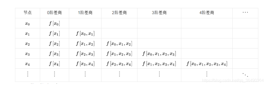
我们把这种叫做差商,0阶均差定义为 $f[x_i]=f(x_i)$ , $n - 1$ 阶差商为：

$f[x_1,x_2,x_3\dots x_n]=\frac{f[x_1,x_2,x_3\dots x_{n-1}]-f[x_2,x_3,x_4\dots x_n]}{x_n-x_1}$
下面是差商表,每次迭代也可重用上一步的结果
在这里插入图片描述
所以最终为
$\begin{aligned} N(x)=& f\left(x_{1}\right)+\\ & f\left[x_{1}, x_{2}\right]\left(x-x_{1}\right)+\\ & f\left[x_{1}, x_{2}, x_{3}\right]\left(x-x_{1}\right)\left(x-x_{2}\right)+\\ & f\left[x_{1}, \ldots, x_{4}\right]\left(x-x_{1}\right)\left(x-x_{2}\right)\left(x-x_{3}\right)+\\ & \ldots \end{aligned}$

以下是代码,可想而知，虽然Newton插值效率提高了，但是也要多出一部分来计算差商

#include<iostream>
#include<stdio.h>
#include<stdlib.h>
using namespace std;
float x[7] = {1.20, 1.24, 1.28, 1.32, 1.36, 1.40};
float y1[7] = {1.09545, 1.11355, 1.13137,1.14891, 1.16619, 1.18322};
float y2[7] = {0.07918, 0.09342, 0.10721, 0.12057, 0.13354, 0.14613};
float xi[6] = {1.22, 1.26, 1.30, 1.34, 1.38};
float diff[10][10];//差商值表
float phi[10];//基函数值
int n=6;

//求差商表，有点像动态规划
void DifferenceQuotient(float *y)
{
  for (int i = 0; i < n;i++)
    diff[i][0] = y[i];
    
  for (int i = 1; i < n;i++)
  {
    for (int j = 1 ; j < i+1;j++)
      diff[i][j] = (diff[i][j - 1] - diff[i-1][j - 1]) / (x[i] - x[i-j]);
  }

}


float Newton(float *y,float cx)
{
  phi[0] = 1;
  float ans = 0;
  for (int i = 1; i < n;i++) //其基函数的值
    phi[i] = phi[i-1]*(cx - x[i-1]);
  
  for (int i = 0; i < n;i++)
    ans += phi[i] * diff[i][i];//多项式求和为最终结果
  
  return ans;
}

int main(){
  DifferenceQuotient(y1);
  for (int i = 0; i < 5;i++)
        printf("当x=%.2f,y1=%.5f\n", xi[i], Newton(y1,xi[i]));

  cout << endl;

  DifferenceQuotient(y2);
  for (int i = 0; i < 5;i++)
        printf("当x=%.2f,y2=%.5f\n", xi[i],Newton(y2,xi[i]));

  system("pause");
}

如果要新增节点，可以增量更新差商表

两者关系

其实我们可以发现两个方法都是通过 $n$ 个点确定了一组 $n$ 个方程的方程组:
$\begin{cases} y_1&=a_0+a_1x_1+a_2x_1^2+\dots+a_nx_1^n\\ y_2&=a_0+a_1x_2+a_2x_2^2+\dots+a_nx_2^n\\ \vdots\\ y_n&=a_0+a_1x_n+a_2x_n^2+\dots+a_nx_n^n\\ \end{cases}$
矩阵形式为 $Y = X A$
$\begin{bmatrix} y_1\\y_2\\ \vdots \\y_n\end{bmatrix}= \begin{bmatrix} 1&x_1&x_1^2&\dots&x_1^n\\1&x_2&x_2^2&\dots&x_2^n\\ \vdots&\vdots&\vdots&\dots&\vdots\\1&x_n&x_n^2&\dots&x_n^n\end{bmatrix} \begin{bmatrix} a_0\\a_1\\ \vdots \\a_n\end{bmatrix}$
系数矩阵 $X$ 为范德蒙行列式,则 $|X|\not =0$ ,因此可以得出其解 $A$ 唯一,故最终确定的多项式唯一,即两者等效.Largrane法较为简单，而Newton法在需要新增节点时可以保持很好的效率。