Logistic Regression with a Neural Network mindset

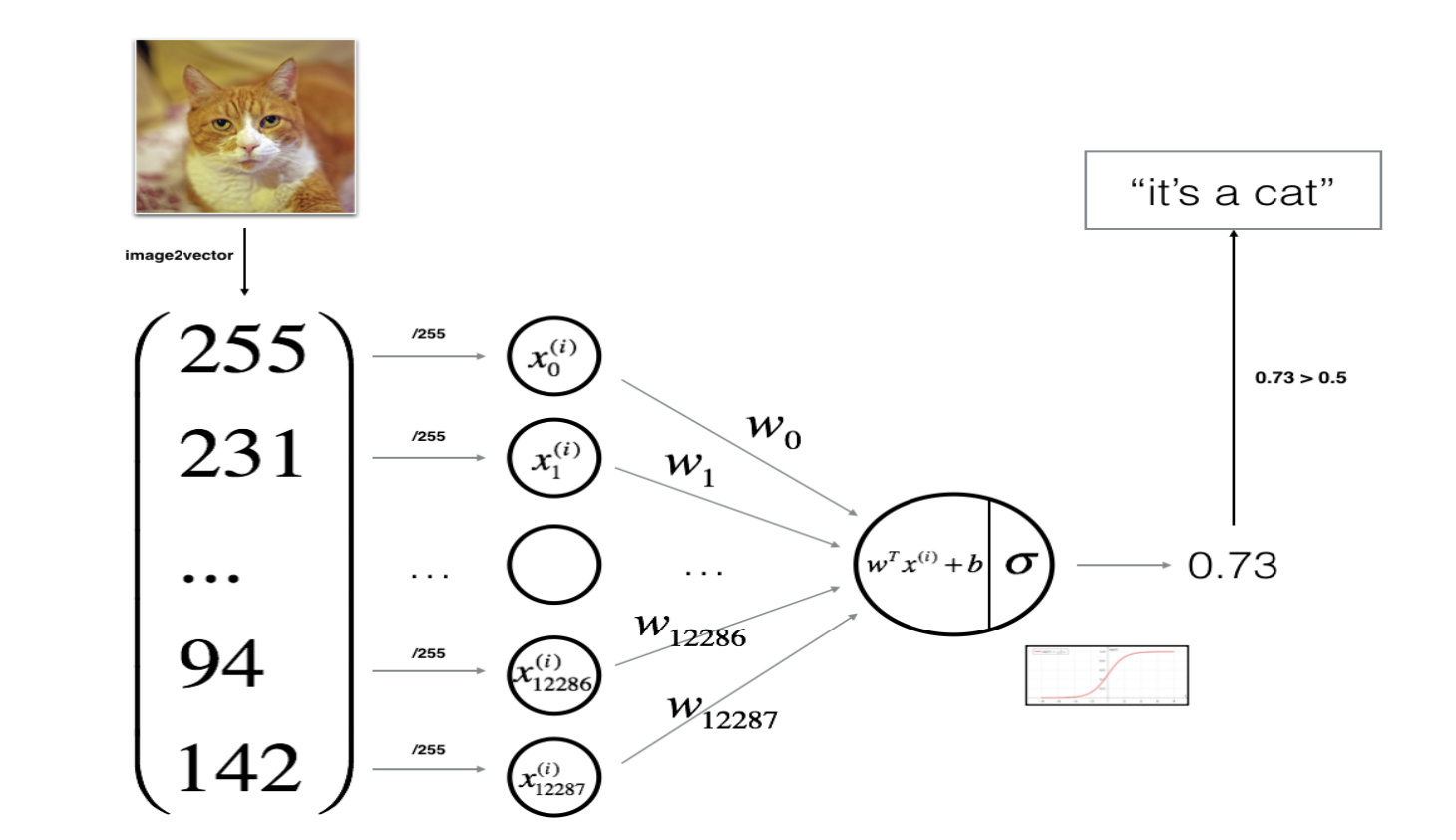
Logistic Regression with a Neural Network mindset

General Architecture of the learning algorithm

It’s time to design a simple algorithm to distinguish cat images from non-cat images.

I will build a Logistic Regression, using a Neural Network mindset. The following Figure explains why Logistic Regression is actually a very simple Neural Network!

Mathematical expression of the algorithm:

For one example Missing superscript or subscript argument x^{(i)} :

$$z^{(i)}=w^T{x}^{(i)}b\text{\hspace{1em}(1)}$$

$${\hat{y}}^{(i)}=a^{(i)}=sigmoid(z^{(i)})\text{\hspace{1em}(2)}$$

$$\mathcal{L}(a^{(i)},y^{(i)})=-y^{(i)}\log (a^{(i)})-(1-y^{(i)})\log (1-a^{(i)})\text{\hspace{1em}(3)}$$

The cost is then computed by summing over all training examples:
$$J=\frac{1}{m}\sum _{i=1}^m\mathcal{L}(a^{(i)},y^{(i)})\text{\hspace{1em}(4)}$$

Key steps:
In this exercise, I will carry out the following steps:

- Initialize the parameters of the model

• Learn the parameters for the model by minimizing the cost
• Use the learned parameters to make predictions (on the test set)
• Analyse the results and conclude

Building the parts of algorithm

The main steps for building a Neural Network are:

1. Define the model structure (such as number of input features)
2. Initialize the model’s parameters
3. Loop:
   • Calculate current loss (forward propagation)
   • Calculate current gradient (backward propagation)
   • Update parameters (gradient descent)

You often build 1-3 separately and integrate them into one function we call model().

Helper functions

sigmoid

Using code from “Python Basics”, implement sigmoid(). As we seen in the figure above, I will compute $sigmoid(w^{T}xb)=\frac{1}{1e^{-(w^{T}xb)}}$ to make predictions. I will use np.exp().

def sigmoid(z):
    """
    Compute the sigmoid of z

    Arguments:
    z -- A scalar or numpy array of any size.

    Return:
    s -- sigmoid(z)
    """

    ### START CODE HERE ### (≈ 1 line of code)
    s = 1 / (1   np.exp(-z))
    ### END CODE HERE ###

    return s

initialize_with_zeros

def initialize_with_zeros(dim):
    """
    This function creates a vector of zeros of shape (dim, 1) for w and initializes b to 0.
    
    Argument:
    dim -- size of the w vector we want (or number of parameters in this case)
    
    Returns:
    w -- initialized vector of shape (dim, 1)
    b -- initialized scalar (corresponds to the bias)
    """

    ### START CODE HERE ### (≈ 1 line of code)
    w = np.zeros(shape=(dim, 1))
    b = 0
    ### END CODE HERE ###

    assert (w.shape == (dim, 1))
    assert (isinstance(b, float) or isinstance(b, int))

    return w, b

Forward and Backward propagation

Now that our parameters are initialized, we can do the “forward” and “backward” propagation steps for learning the parameters.

Exercise: Implement a function propagate() that computes the cost function and its gradient.

Hints:

Forward Propagation:

• I get X
• I compute $A=\sigma (w^{T}Xb)=(a^{(1)},a^{(2)},...,a^{(m-1)},a^{(m)})$
• I calculate the cost function: $J=-\frac{1}{m}{\sum }_{i=1}^m{y}^{(i)}\log (a^{(i)})(1-y^{(i)})\log (1-a^{(i)})$

Here are the two formulas I will be using:

$$\frac{\partial J}{\partial w}=\frac{1}{m}X(A-Y{)}^T\text{\hspace{1em}(5)}$$
$$\frac{\partial J}{\partial b}=\frac{1}{m}\sum _{i=1}^m(a^{(i)}-y^{(i)})\text{\hspace{1em}(6)}$$

def propagate(w, b, X, Y):
    """
    Implement the cost function and its gradient for the propagation explained above

    Arguments:
    w -- weights, a numpy array of size (num_px * num_px * 3, 1)
    b -- bias, a scalar
    X -- data of size (num_px * num_px * 3, number of examples)
    Y -- true "label" vector (containing 0 if non-cat, 1 if cat) of size (1, number of examples)

    Return:
    cost -- negative log-likelihood cost for logistic regression
    dw -- gradient of the loss with respect to w, thus same shape as w
    db -- gradient of the loss with respect to b, thus same shape as b
    
    Tips:
    - Write your code step by step for the propagation. np.log(), np.dot()
    """

    m = X.shape[1]

    # FORWARD PROPAGATION (FROM X TO COST)
    ### START CODE HERE ### (≈ 2 lines of code)
    A = sigmoid(np.dot(w.T, X)   b)  # compute activation
    cost = -(1 / m) * np.sum(Y * np.log(A)   (1 - Y) * np.log(1 - A), axis=1)  # compute cost
    ### END CODE HERE ###

    # BACKWARD PROPAGATION (TO FIND GRAD)
    ### START CODE HERE ### (≈ 2 lines of code)
    dw = (1 / m) * np.dot(X, (A - Y).T)
    db = (1 / m) * np.sum(A - Y)
    ### END CODE HERE ###

    assert (dw.shape == w.shape)
    assert (db.dtype == float)
    cost = np.squeeze(cost)
    assert (cost.shape == ())

    grads = {"dw": dw,
             "db": db}

    return grads, cost

Optimization

• I have initialized our parameters.
• We are also able to compute a cost function and its gradient.
• Now, I want to update the parameters using gradient descent.

Exercise: Write down the optimization function. The goal is to learn w and b by minimizing the cost function J. For a parameter \theta, the update rule is $\theta =\theta -\alpha d\theta$, where $\alpha$ is the learning rate.

def optimize(w, b, X, Y, num_iterations, learning_rate, print_cost=False):
    """
    This function optimizes w and b by running a gradient descent algorithm
    
    Arguments:
    w -- weights, a numpy array of size (num_px * num_px * 3, 1)
    b -- bias, a scalar
    X -- data of shape (num_px * num_px * 3, number of examples)
    Y -- true "label" vector (containing 0 if non-cat, 1 if cat), of shape (1, number of examples)
    num_iterations -- number of iterations of the optimization loop
    learning_rate -- learning rate of the gradient descent update rule
    print_cost -- True to print the loss every 100 steps
    
    Returns:
    params -- dictionary containing the weights w and bias b
    grads -- dictionary containing the gradients of the weights and bias with respect to the cost function
    costs -- list of all the costs computed during the optimization, this will be used to plot the learning curve.
    
    Tips:
    You basically need to write down two steps and iterate through them:
        1) Calculate the cost and the gradient for the current parameters. Use propagate().
        2) Update the parameters using gradient descent rule for w and b.
    """

    costs = []

    for i in range(num_iterations):

        # Cost and gradient calculation (≈ 1-4 lines of code)
        ### START CODE HERE ### 
        grads, cost = propagate(w, b, X, Y)
        ### END CODE HERE ###

        # Retrieve derivatives from grads
        dw = grads["dw"]
        db = grads["db"]

        # update rule (≈ 2 lines of code)
        ### START CODE HERE ###
        w = w - learning_rate * dw
        b = b - learning_rate * db
        ### END CODE HERE ###

        # Record the costs
        if i % 100 == 0:
            costs.append(cost)

        # Print the cost every 100 training iterations
        if print_cost and i % 100 == 0:
            print("Cost after iteration %i: %f" % (i, cost))

    params = {"w": w,
              "b": b}

    grads = {"dw": dw,
             "db": db}

    return params, grads, costs

predict

Exercise: The previous function will output the learned w and b. We are able to use w and b to predict the labels for a dataset X. Implement the predict() function. There are two steps to computing predictions:

1. Calculate $\hat{Y}=A=\sigma (w^{T}Xb)$
2. Convert the entries of a into 0 (if activation <= 0.5) or 1 (if activation > 0.5), stores the predictions in a vector Y_prediction. If you wish, you can use an if/else statement in a for loop (though there is also a way to vectorize this).

def predict(w, b, X):
    '''
    Predict whether the label is 0 or 1 using learned logistic regression parameters (w, b)
    
    Arguments:
    w -- weights, a numpy array of size (num_px * num_px * 3, 1)
    b -- bias, a scalar
    X -- data of size (num_px * num_px * 3, number of examples)
    
    Returns:
    Y_prediction -- a numpy array (vector) containing all predictions (0/1) for the examples in X
    '''

    m = X.shape[1]
    Y_prediction = np.zeros((1, m))
    w = w.reshape(X.shape[0], 1)

    # Compute vector "A" predicting the probabilities of a cat being present in the picture
    ### START CODE HERE ### (≈ 1 line of code)
    A = sigmoid(np.dot(w.T, X)   b)
    ### END CODE HERE ###

    for i in range(A.shape[1]):

        # Convert probabilities A[0,i] to actual predictions p[0,i]
        ### START CODE HERE ### (≈ 4 lines of code)
        if A[0][i] < 0.5:
            Y_prediction[0][i] = 0
        else:
            Y_prediction[0][i] = 1

        ### END CODE HERE ###

    assert (Y_prediction.shape == (1, m))

    return Y_prediction

What to remember

We’ve implemented several functions that:

• Initialize (w,b)
• Optimize the loss iteratively to learn parameters (w,b):
  • computing the cost and its gradient
  • updating the parameters using gradient descent
• Use the learned (w,b) to predict the labels for a given set of examples

Merge all functions into a model

You will now see how the overall model is structured by putting together all the building blocks (functions implemented in the previous parts) together, in the right order.

Exercise: Implement the model function. Use the following notation:

- Y_prediction_test for your predictions on the test set

• Y_prediction_train for your predictions on the train set
• w, costs, grads for the outputs of optimize()

def model(X_train, Y_train, X_test, Y_test, num_iterations=2000, learning_rate=0.5, print_cost=False):
    """
    Builds the logistic regression model by calling the function you've implemented previously
    
    Arguments:
    X_train -- training set represented by a numpy array of shape (num_px * num_px * 3, m_train)
    Y_train -- training labels represented by a numpy array (vector) of shape (1, m_train)
    X_test -- test set represented by a numpy array of shape (num_px * num_px * 3, m_test)
    Y_test -- test labels represented by a numpy array (vector) of shape (1, m_test)
    num_iterations -- hyperparameter representing the number of iterations to optimize the parameters
    learning_rate -- hyperparameter representing the learning rate used in the update rule of optimize()
    print_cost -- Set to true to print the cost every 100 iterations
    
    Returns:
    d -- dictionary containing information about the model.
    """

    ### START CODE HERE ###

    # initialize parameters with zeros (≈ 1 line of code)
    w, b = initialize_with_zeros(X_train.shape[0])

    # Gradient descent (≈ 1 line of code)
    params, grads, costs = optimize(w, b, X_train, Y_train, num_iterations=num_iterations, learning_rate=learning_rate,
                                    print_cost=print_cost)

    # Retrieve parameters w and b from dictionary "parameters"
    w = params["w"]
    b = params["b"]

    # Predict test/train set examples (≈ 2 lines of code)
    Y_prediction_test = predict(w, b, X_test)
    Y_prediction_train = predict(w, b, X_train)

    ### END CODE HERE ###

    # Print train/test Errors
    print("train accuracy: {} %".format(100 - np.mean(np.abs(Y_prediction_train - Y_train)) * 100))
    print("test accuracy: {} %".format(100 - np.mean(np.abs(Y_prediction_test - Y_test)) * 100))

    d = {"costs": costs,
         "Y_prediction_test": Y_prediction_test,
         "Y_prediction_train": Y_prediction_train,
         "w": w,
         "b": b,
         "learning_rate": learning_rate,
         "num_iterations": num_iterations}

    return d

train

d = model(train_set_x, train_set_y, test_set_x, test_set_y, num_iterations=2000, learning_rate=0.005, print_cost=True)

test our image

## START CODE HERE ## (PUT YOUR IMAGE NAME) 
my_image = "my_image.jpg"   # change this to the name of your image file 
## END CODE HERE ##

# We preprocess the image to fit your algorithm.
fname = "images/"   my_image
image = np.array(ndimage.imread(fname, flatten=False))
my_image = scipy.misc.imresize(image, size=(num_px,num_px)).reshape((1, num_px*num_px*3)).T
my_predicted_image = predict(d["w"], d["b"], my_image)

plt.imshow(image)
print("y = "   str(np.squeeze(my_predicted_image))   ", your algorithm predicts a \""   classes[int(np.squeeze(my_predicted_image)),].decode("utf-8")    "\" picture.")