


2.1.4 图像教程
使用Matplotlib绘制图像的简短教程。
启动命令
首先,让我们开始IPython。它是对标准Python提示符的最优秀的增强,它与Matplotlib结合得特别好。直接在shell上启动lPython,或者使用Jupyter笔记本(其中IPython作为运行的内核)。
启动lPython后,我们现在需要连接到GUI事件循环。这将告诉IPython在哪里(以及如何)显示图形。要连接到GUI循环,请在IPython提示符下执行%matplotlib命令。在IPython关于GUI事件循环的文档(IPython’s documentation on GUI event loops)中,有更详细的说明。
lf you’re using Jupyter Notebook, the same commands are available, but people commonly use a specificargument to the %matplotlib magic:
如果您使用的是Jupyter Notebook,也可以使用相同的命令,但人们通常会使用%matplotlib来设置特定参数:
In [1]: %matplotlib inline
这将打开内联绘图,其中的绘图将出现在您的notebook.。这对于互动性有着重要的含义。对于内联绘图,输出绘图的单元格下面的单元格中的命令不会影响绘图。例如,从创建绘图的单元格下面的单元格中更改颜色图是不可能的。但是,对于其他后端(如Qt5),打开单独窗口的其他后端,在创建图形的单元格下面的单元格将更改绘图——它是内存中的活动对象。
本教程将使用Matplotlitb的命令式绘图接口pyplote。该接口维护全局状态,对于快速方便地进行各种绘图设置的实验非常有用。另一种是面向对象的接口,它也非常强大,通常更适合于大型应用程序的开发。如果您想了解面向对象的界面,最好的起点是我们的Usage Guide。
现在,让我们开始使用命令式方法:
import matplotlib.pyplot as plt
import matplotlib.image as mpimg
将图像数据移植到Numpy阵列
Matplotlib依赖于Pillow库来加载图像数据。下面是我们将要使用的图像:
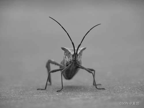
这是一个24位的RGB PNG图像(R,G,B各8位),取决于您从何处获得数据,您最可能遇到的其他类型的图像是RGBA图像,它允许透明性,或单通道灰度(亮度)图像。把stinkbug.png下载到你的电脑上完成剩下的教程。
现在我们输出图像数据:
img = mpimg.imread('../../doc/_static/stinkbug.png')
print(img)
输出:
[[[0.40784314 0.40784314 0.40784314]
[0.40784314 0.40784314 0.40784314]
[0.40784314 0.40784314 0.40784314]
...
[0.42745098 0.42745098 0.42745098]
[0.42745098 0.42745098 0.42745098]
[0.42745098 0.42745098 0.42745098]]
[[0.4117647 0.4117647 0.4117647 ]
[0.4117647 0.4117647 0.4117647 ]
[0.4117647 0.4117647 0.4117647 ]
...
 [0.42745098 0.42745098 0.42745098]
[0.42745098 0.42745098 0.42745098]
[0.42745098 0.42745098 0.42745098]]
[[0.41960785 0.41960785 0.41960785]
[0.41568628 0.41568628 0.41568628]
[0.41568628 0.41568628 0.41568628]
...
[0.43137255 0.43137255 0.43137255]
[0.43137255 0.43137255 0.43137255]
[0.43137255 0.43137255 0.43137255]]
...
[[0.4392157 0.4392157 0.4392157 ]
[0.43529412 0.43529412 0.43529412]
[0.43137255 0.43137255 0.43137255]
...
[0.45490196 0.45490196 0.45490196]
[0.4509804 0.4509804 0.4509804 ]
[0.4509804 0.4509804 0.4509804 ]]
[[0.44313726 0.44313726 0.44313726]
[0.44313726 0.44313726 0.44313726]
[0.4392157 0.4392157 0.4392157 ]
...
[0.4509804 0.4509804 0.4509804 ]
[0.44705883 0.44705883 0.44705883]
[0.44705883 0.44705883 0.44705883]]
[[0.44313726 0.44313726 0.44313726]
[0.4509804 0.4509804 0.4509804 ]
[0.4509804 0.4509804 0.4509804 ]
...
[0.44705883 0.44705883 0.44705883]
[0.44705883 0.44705883 0.44705883]
[0.44313726 0.44313726 0.44313726]]]
注意那里的dtype-Float32没?Matplotlib已经将8位数据,从每个通道重新标度到0.0到1.0之间的浮点数据库。作为side的注释,Pillow可以使用的唯一数据类型是uint 8。Matplotlib可以处理float32和uint 8,但是除png之外的任何格式的图像读/写仅限于uint 8数据。为什么是8位?大多数显示器只能呈现8位每通道价值的颜色分级。为什么他们只能渲染8位/通道?因为这是人类眼睛所能看到的。更多信息请参阅(从照片的角度来看):发光景观比特深度教程。
每个内部列表表示一个像素。在这里,有一个RGB图像,有3个值。因为它是黑色和白色图像,R、G和B都是相似的。一个RGBA(其中A是alpha,或透明度),每个内部列表有4个值,一个简单的亮度图像只有一个值(因此它只是一个二维数组,而不是一个3D数组)。对于RGB和RGBA图像,Matplotlib支持float32和uint 8数据类型。
将numpy数组绘制为图像
因此,您可以将数据保存在numpy数组中(通过导入数据或生成数据)。我们来渲染吧。在Matplotlib,这是使用imshow()函数执行的。在这里,我们将抓取图像对象。这个对象为您提供了一种从提示符中操作绘图的简单方法。
imgplot = plt.imshow(img)
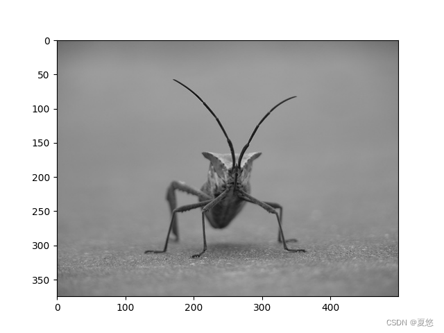
您还可以绘制任意数字数组。
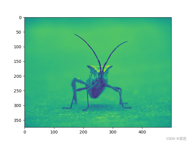
伪彩色算法在图像绘制中的应用
伪彩色可以是一个有用的工具,以增强对比度和可视化您的数据更容易。这是特别有用的,当你用投影仪做你的数据演示时,它们的对比通常很差。
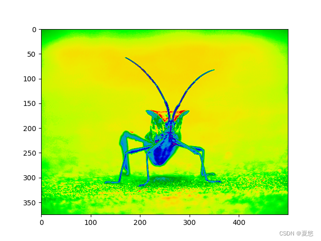
伪彩色只与单通道、灰度、亮度图像相关.我们目前有一个RGB映像,因为SinceR、G和B都是相似的(请参阅上面或在您的数据中),我们只需选择我们的数据中的一个通道:
lum_img = img[:, :, 0]
# 这是数组切片。您可以在“Numpy教程”中阅读更多信息
# <https://docs.scipy.org/doc/numpy/user/quickstart.html>`_.
plt.imshow(lum_img)
输出:
<matplotlib.image.AxesImage object at 0x7f5eff0121f0>
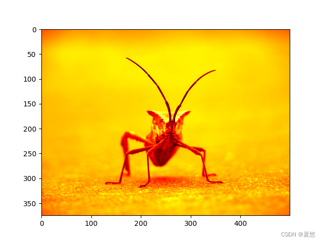
现在,对于亮度(2D,无颜色)图像,将应用默认的颜色映射(也称为查找表,LUT)。默认情况称为病毒,有很多其他的选择。
plt.imshow(lum_img, cmap="hot")
输出:
<matplotlib.image.AxesImage object at 0x7f5f0893cbb0>
请注意,您还可以使用set_cmap()方法更改现有绘图对象上的颜色贴图:
imgplot = plt.imshow(lum_img)
imgplot.set_cmap('nipy_spectral')
注意:但是,请记住,在带有内联后端的Jupyter Notebook中,您不能对已经呈现的图形进行更改。如果在一个单元格中在这里创建图像,则不能在后一个单元格中调用set_cmap(),并期望更改先前的绘图。确保在一个单元格中一起输入这些命令。plt命令不会更改以前的单元格中的图表。
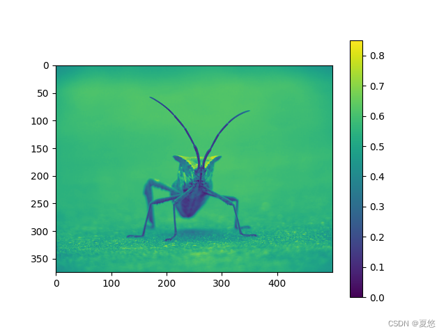
彩色标度基准
了解颜色所代表的价值是有帮助的。我们可以通过在您的图形中添加一个颜色条来做到这一点:
imgplot = plt.imshow(lum_img)
plt.colorbar()
输出:
<matplotlib.colorbar.Colorbar object at 0x7f5efdc22880>
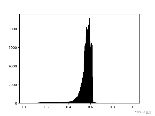
检查特定的数据范围
有时你想增强图像中的对比度,或者在特定区域扩大对比度,同时牺牲颜色变化不大或无关紧要的细节。为了创建图像数据的直方图,我们使用hist()函数。
plt.hist(lum_img.ravel(), bins=256, range=(0.0, 1.0), fc='k', ec='k')
输出:
(array([2.000e+00, 2.000e+00, 3.000e+00, 3.000e+00, 2.000e+00, 2.000e+00,
3.000e+00, 1.000e+00, 7.000e+00, 9.000e+00, 7.000e+00, 2.000e+00,
7.000e+00, 1.000e+01, 1.100e+01, 1.500e+01, 1.400e+01, 2.700e+01,
2.100e+01, 2.400e+01, 1.400e+01, 3.100e+01, 2.900e+01, 2.800e+01,
2.400e+01, 2.400e+01, 4.000e+01, 2.600e+01, 5.200e+01, 3.900e+01,
5.700e+01, 4.600e+01, 8.400e+01, 7.600e+01, 8.900e+01, 8.000e+01,
1.060e+02, 1.130e+02, 1.120e+02, 9.000e+01, 1.160e+02, 1.090e+02,
1.270e+02, 1.350e+02, 9.800e+01, 1.310e+02, 1.230e+02, 1.110e+02,
1.230e+02, 1.160e+02, 1.010e+02, 1.170e+02, 1.000e+02, 1.010e+02,
9.000e+01, 1.060e+02, 1.260e+02, 1.040e+02, 1.070e+02, 1.110e+02,
1.380e+02, 1.000e+02, 1.340e+02, 1.210e+02, 1.400e+02, 1.320e+02,
1.390e+02, 1.160e+02, 1.330e+02, 1.180e+02, 1.080e+02, 1.170e+02,
1.280e+02, 1.200e+02, 1.210e+02, 1.100e+02, 1.160e+02, 1.180e+02,
9.700e+01, 9.700e+01, 1.140e+02, 1.070e+02, 1.170e+02, 8.700e+01,
1.070e+02, 9.800e+01, 1.040e+02, 1.120e+02, 1.110e+02, 1.180e+02,
1.240e+02, 1.340e+02, 1.200e+02, 1.410e+02, 1.520e+02, 1.360e+02,
1.610e+02, 1.380e+02, 1.620e+02, 1.570e+02, 1.350e+02, 1.470e+02,
1.690e+02, 1.710e+02, 1.820e+02, 1.980e+02, 1.970e+02, 2.060e+02,
2.160e+02, 2.460e+02, 2.210e+02, 2.520e+02, 2.890e+02, 3.450e+02,
3.620e+02, 3.760e+02, 4.480e+02, 4.630e+02, 5.170e+02, 6.000e+02,
6.200e+02, 6.410e+02, 7.440e+02, 7.120e+02, 8.330e+02, 9.290e+02,
1.061e+03, 1.280e+03, 1.340e+03, 1.638e+03, 1.740e+03, 1.953e+03,
2.151e+03, 2.290e+03, 2.440e+03, 2.758e+03, 2.896e+03, 3.384e+03,
4.332e+03, 5.584e+03, 6.197e+03, 6.422e+03, 6.404e+03, 7.181e+03,
8.196e+03, 7.968e+03, 7.474e+03, 7.926e+03, 8.460e+03, 8.091e+03,
9.148e+03, 8.563e+03, 6.747e+03, 6.074e+03, 6.328e+03, 5.291e+03,
6.472e+03, 6.268e+03, 2.864e+03, 3.760e+02, 1.620e+02, 1.180e+02,
1.270e+02, 9.500e+01, 7.600e+01, 8.200e+01, 6.200e+01, 6.700e+01,
5.600e+01, 5.900e+01, 4.000e+01, 4.200e+01, 3.000e+01, 3.400e+01,
3.200e+01, 4.300e+01, 4.200e+01, 2.300e+01, 2.800e+01, 1.900e+01,
2.200e+01, 1.600e+01, 1.200e+01, 1.800e+01, 9.000e+00, 1.000e+01,
1.700e+01, 5.000e+00, 2.100e+01, 1.300e+01, 8.000e+00, 1.200e+01,
1.000e+01, 8.000e+00, 8.000e+00, 5.000e+00, 1.300e+01, 6.000e+00,
3.000e+00, 7.000e+00, 6.000e+00, 2.000e+00, 1.000e+00, 5.000e+00,
3.000e+00, 3.000e+00, 1.000e+00, 1.000e+00, 1.000e+00, 5.000e+00,
0.000e+00, 1.000e+00, 3.000e+00, 0.000e+00, 1.000e+00, 1.000e+00,
2.000e+00, 1.000e+00, 0.000e+00, 0.000e+00, 0.000e+00, 0.000e+00,
0.000e+00, 0.000e+00, 0.000e+00, 0.000e+00, 0.000e+00, 0.000e+00,
0.000e+00, 0.000e+00, 0.000e+00, 0.000e+00, 0.000e+00, 0.000e+00,
0.000e+00, 0.000e+00, 0.000e+00, 0.000e+00, 0.000e+00, 0.000e+00,
0.000e+00, 0.000e+00, 0.000e+00, 0.000e+00, 0.000e+00, 0.000e+00,
0.000e+00, 0.000e+00, 0.000e+00, 0.000e+00, 0.000e+00, 0.000e+00,
0.000e+00, 0.000e+00, 0.000e+00, 0.000e+00]), array([0. , 0.
↪00390625, 0.0078125 , 0.01171875, 0.015625 ,
0.01953125, 0.0234375 , 0.02734375, 0.03125 , 0.03515625,
0.0390625 , 0.04296875, 0.046875 , 0.05078125, 0.0546875 ,
0.05859375, 0.0625 , 0.06640625, 0.0703125 , 0.07421875,
0.078125 , 0.08203125, 0.0859375 , 0.08984375, 0.09375 ,
0.09765625, 0.1015625 , 0.10546875, 0.109375 , 0.11328125,
0.1171875 , 0.12109375, 0.125 , 0.12890625, 0.1328125 ,
0.13671875, 0.140625 , 0.14453125, 0.1484375 , 0.15234375,
0.15625 , 0.16015625, 0.1640625 , 0.16796875, 0.171875 ,
0.17578125, 0.1796875 , 0.18359375, 0.1875 , 0.19140625,
0.1953125 , 0.19921875, 0.203125 , 0.20703125, 0.2109375 ,
0.21484375, 0.21875 , 0.22265625, 0.2265625 , 0.23046875,
0.234375 , 0.23828125, 0.2421875 , 0.24609375, 0.25 ,
0.25390625, 0.2578125 , 0.26171875, 0.265625 , 0.26953125,
0.2734375 , 0.27734375, 0.28125 , 0.28515625, 0.2890625 ,
0.29296875, 0.296875 , 0.30078125, 0.3046875 , 0.30859375,
0.3125 , 0.31640625, 0.3203125 , 0.32421875, 0.328125 ,
0.33203125, 0.3359375 , 0.33984375, 0.34375 , 0.34765625,
0.3515625 , 0.35546875, 0.359375 , 0.36328125, 0.3671875 ,
0.37109375, 0.375 , 0.37890625, 0.3828125 , 0.38671875,
0.390625 , 0.39453125, 0.3984375 , 0.40234375, 0.40625 ,
0.41015625, 0.4140625 , 0.41796875, 0.421875 , 0.42578125,
0.4296875 , 0.43359375, 0.4375 , 0.44140625, 0.4453125 ,
0.44921875, 0.453125 , 0.45703125, 0.4609375 , 0.46484375,
0.46875 , 0.47265625, 0.4765625 , 0.48046875, 0.484375 ,
0.48828125, 0.4921875 , 0.49609375, 0.5 , 0.50390625,
0.5078125 , 0.51171875, 0.515625 , 0.51953125, 0.5234375 ,
0.52734375, 0.53125 , 0.53515625, 0.5390625 , 0.54296875,
0.546875 , 0.55078125, 0.5546875 , 0.55859375, 0.5625 ,
0.56640625, 0.5703125 , 0.57421875, 0.578125 , 0.58203125,
0.5859375 , 0.58984375, 0.59375 , 0.59765625, 0.6015625 ,
0.60546875, 0.609375 , 0.61328125, 0.6171875 , 0.62109375,
0.625 , 0.62890625, 0.6328125 , 0.63671875, 0.640625 ,
0.64453125, 0.6484375 , 0.65234375, 0.65625 , 0.66015625,
0.6640625 , 0.66796875, 0.671875 , 0.67578125, 0.6796875 ,
0.68359375, 0.6875 , 0.69140625, 0.6953125 , 0.69921875,
0.703125 , 0.70703125, 0.7109375 , 0.71484375, 0.71875 ,
0.72265625, 0.7265625 , 0.73046875, 0.734375 , 0.73828125,
0.7421875 , 0.74609375, 0.75 , 0.75390625, 0.7578125 ,
0.76171875, 0.765625 , 0.76953125, 0.7734375 , 0.77734375,
0.78125 , 0.78515625, 0.7890625 , 0.79296875, 0.796875 ,
0.80078125, 0.8046875 , 0.80859375, 0.8125 , 0.81640625,
0.8203125 , 0.82421875, 0.828125 , 0.83203125, 0.8359375 ,
0.83984375, 0.84375 , 0.84765625, 0.8515625 , 0.85546875,
0.859375 , 0.86328125, 0.8671875 , 0.87109375, 0.875 ,
0.87890625, 0.8828125 , 0.88671875, 0.890625 , 0.89453125,
0.8984375 , 0.90234375, 0.90625 , 0.91015625, 0.9140625 ,
0.91796875, 0.921875 , 0.92578125, 0.9296875 , 0.93359375,
0.9375 , 0.94140625, 0.9453125 , 0.94921875, 0.953125 ,
0.95703125, 0.9609375 , 0.96484375, 0.96875 , 0.97265625,
0.9765625 , 0.98046875, 0.984375 , 0.98828125, 0.9921875 ,
0.99609375, 1. ], dtype=float32), <BarContainer object of 256␣
↪artists>)
Most often, the “interesting” part of the image is around the peak, and you can get extra contrast by clippingthe regions above and/or below the peak. In our histogram, it looks like there’s not much useful informationin the high end (not many white things in the image).Let’s adjust the upper limit, so that we effectively"zoom in on" part of the histogram. We do this by passing the clim argument to imshow.You could also dothis by calling the set_clim ( ) method of the image plot object, but make sure that you do so in the samecell as your plot command when working with the Jupyter Notebook - it will not change plots from earliercells.
最常见的情况是,图像的“有趣”部分在峰值周围,您可以通过剪裁峰值上方和/或下面的区域来获得额外的对比度。在我们的直方图中,高端(图像中白色的东西不多)似乎没有多少有用的信息。让我们调整上限,这样我们就可以有效地“放大”直方图的一部分。我们通过将clim参数传递给imshow来实现这一点,您也可以通过调用图像绘图对象的set_clim()方法来做到这一点,但是在使用Jupyter Notebook时,请确保在相同的单元格中作为绘图命令这样做——它不会从早期的单元格中更改绘图。
您可以在调用绘图时指定clim:
imgplot = plt.imshow(lum_img, clim=(0.0, 0.7))
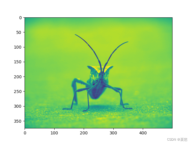
也可以使用返回的对象指定clim:
fig = plt.figure()
ax = fig.add_subplot(1, 2, 1)
imgplot = plt.imshow(lum_img)
ax.set_title('Before')
plt.colorbar(ticks=[0.1, 0.3, 0.5, 0.7], orientation='horizontal')
ax = fig.add_subplot(1, 2, 2)
imgplot = plt.imshow(lum_img)
imgplot.set_clim(0.0, 0.7)
ax.set_title('After')
plt.colorbar(ticks=[0.1, 0.3, 0.5, 0.7], orientation='horizontal')

输出:
<matplotlib.colorbar.Colorbar object at 0x7f5eff8a96a0>
阵列插补方案
根据不同的数学家方案,插值计算一个像素的颜色或值应该是什么时,比如当您调整图像大小时,像素数会发生变化。但您需要相同的信息,因为像素是离散的,所以就会有缺失部分。插值填充了空间,这就是为什么你的图像有时看起来十分模糊。当你放大它们时,当原始图像和扩展图像之间的差异更大时,效果会更明显。我们把图形缩缩小的时候,我们实际上是在丢弃像素,只保留少量的选择。现在,当我们绘制它时,数据会被放大到屏幕上的大小。旧的像素不再存在,计算机必须绘制像素来填充这个空间。
我们将使用用来加载映像的Pillow库来调整图像的大小。
from PIL import Image
img = Image.open('../../doc/_static/stinkbug.png')
img.thumbnail((64, 64), Image.ANTIALIAS) # 在适当的位置调整图像大小
imgplot = plt.imshow(img)

这里我们有默认的插值,双线性,因为我们没有给出任何插值论证。
让我们试试其他的,这里是“最近的”,它不做插值。
imgplot = plt.imshow(img, interpolation="nearest")

双立方:
imgplot = plt.imshow(img, interpolation="bicubic")
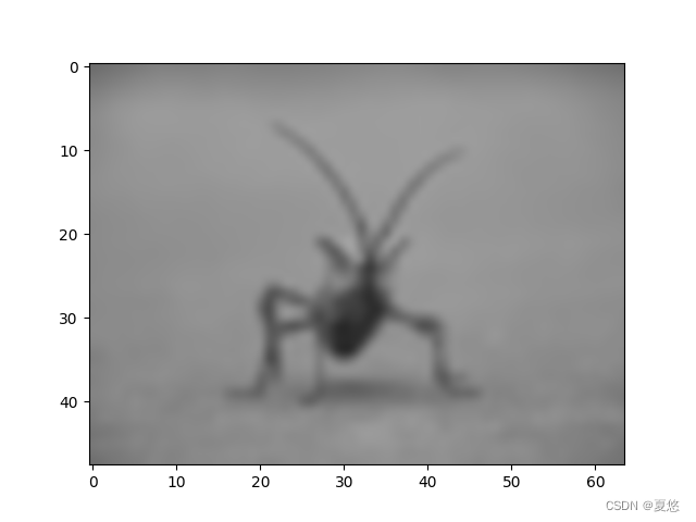
双立方插值通常用于放大照片。人们更喜欢模糊而不是像素化。脚本的总运行时间:(0分6.876秒)


 5007
5007


 被折叠的 条评论
为什么被折叠?
被折叠的 条评论
为什么被折叠?
 到【灌水乐园】发言


