Randomized Algorithms随机算法(Introduction to Algorithms, 算法导论，CLRS)学习笔记

Randomized Algorithms

• Las Vegas Algorithm for quick sort

• Monte Carlo Algorithm for find min cut

• The quick sort:

  • Best case: each time the chose pivot is in the middle; $O(n\log n)$;
  • Worst case: in a sorted list, each time the chosen pivot is in the beginning; $O(n^2)$

1. Random quicksort(Las Vegas Algorithm)

• Always return the right answer or none, but the running time is not sure.

randomly choose the pivot

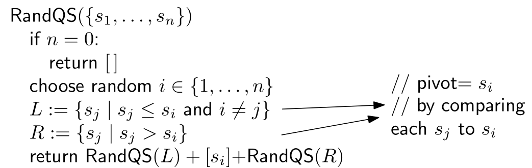
Lemma: RandQS sorts the numbers. Proof: induction on $n$.

• Lucky case: $s_i$ is always the median: $O(n\log n)$

• Unlucky case: $s_i$ is always the minimum: $O(n^2)$

1.3 Average case analysis

Theorem: $E[X]=O(n\log n)$

Proof:

Let $S_1,S_2,...,S_n$ be the numbers in sorted order, and for example:
$$(s_1,s_2,...s_5)=(3,2,1,5,4)$$ and $(S_1,S_2,...,S_5)=(1,2,3,4,5)$

Let $X_{ij}$ denotes comparison between $S_i$ and $S_j$, and $X_{ij}\in 0,1$:

$$E[X]=E[\sum _{i=1}^n\sum _{j>i}{X}_{ij}]=\sum _{i=1}^n\sum _{j>i}E[X_{ij}]$$

Let $p_{ij}$ denotes the probability that $S_i$ and $S_j$ are compared.

Then $E[X_{ij}]=0\times (1-p_{ij})+1\times p_{ij}=p_{ij}$

We can observe that $S_i$ and $S_j$ are compared if and only if when one of them are the pivot. Then the probability of one of them to be chosen as the pivot: $\frac{2}{j-i+1}=p_{ij}$, (pick 2 elements from the number of $S$ need to be compared in an iteration)

Then $E[X]={\sum }_{i=1}^n{\sum }_{k=2}^{n-i+1}\frac{2}{k}\le {\sum }_{i=1}^n{\sum }_{k=1}^n\frac{2}{k}=2n{\sum }_{k=1}^n\frac{1}{k}=2n{H}_n$;

by integration, we can know that $H_n-1\le {\int }_1^n\frac{1}{x}dx=ln(n)$, then $H_n=O(\log n)$; and $E[X]=O(n\log n)$.

2. Randomized min-cut

• Monte Carlo Algorithm, might give the wrong answer

Given: Graph $G=(V,E),|V|\ge 2$.

Find: Min. set of edges $C\subseteq E$, s.t. $G-C$ is disconnected.

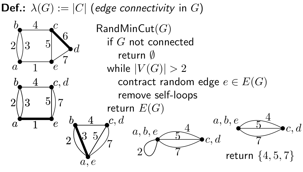
2.1Lemma: RandMinCut(G) returns a cut.

Proof: If $C$ is not a cut, there is path $\pi$ in the original graph $G$ from $u\in V_1$ to $v\in V_2$ that are not in $C$, but we have removed all edges of $\pi$. Contradiction!

2.2Probability of min-cut

Theorem: For any min-cut $C$, $$Pr[RandMinCutreturnsC]\ge \frac{2}{n(n-1)}$$

Proof:

• Define: $G_i=(V_i,E_i)$: graph at the beginning of step i ∈ { 1 , . . . , n − 1 } i\in\{1,...,n-1\} i∈{1,...,n−1}. Step i ∈ { 1 , . . , n − 2 } i\in \{1,..,n-2\} i∈{1,..,n−2} contracts edge $e_i\in E_i$

• $n_i:=|V_i|=n-i+1$ so that $n_1=|V|$;

• Define events: $\epsilon :e_i\notin C$, and ${\epsilon }_j:={\cap }_{i=1}^{j=1}{\epsilon }_i$

• Need to show: $Pr[{\epsilon }_{<n-1}]\ge \frac{2}{n(n-1)}$

• Since in each step, the event that we would not make a mistake is independent, $Pr[{\epsilon }_1|{\epsilon }_{<1}]=Pr[{\epsilon }_1]$, and $Pr[{\epsilon }_{<3}]=Pr[{\epsilon }_2|{\epsilon }_{<2}]=Pr[{\epsilon }_2]Pr[{\epsilon }_1|{\epsilon }_{<1}]$

• Due to this, we know that: $Pr[{\epsilon }_{<n-1}]={\prod }_{i=1}^{n-2}Pr[{\epsilon }_i|{\epsilon }_{<i}]$

• Since cut in $G_i$ is also a cut in $G$: $\lambda (G_i)\ge \lambda (G)=|C|$ and $mi{n}_{v\in V_i}d(v)\ge \lambda (G_i)\ge |C|$, where $d(v)$ is the degree of a vertex.

• $|E_i|={\sum }_{v\in V_i}\frac{d(v)}{2}\ge {\sum }_{v\in V_i}\frac{|C|}{2}=\frac{n_i|C|}{2}$

• $Pr[{\bar{\epsilon }}_i|{\epsilon }_{<i}]=\frac{|C|}{|E_i|}\le \frac{|C|}{n_i|C|/2}=\frac{2}{n_i}$

• $Pr[{\epsilon }_i|{\epsilon }_{<i}]=1-Pr[{\bar{\epsilon }}_i|{\epsilon }_{<i}]\ge \frac{n-i-1}{n-i+1}$

• $Pr[{\epsilon }_{<n-1}]={\prod }_{i=1}^{n-2}Pr[{\epsilon }_i|{\epsilon }_{<i}]\ge {\prod }_{i=1}^{n-2}\frac{n-i-1}{n-i+1}=\frac{2}{n(n-1)}$

2.3Analyze the probability

• Tightness: find a min cut in a circle: $C_n^2=\frac{n(n-1)}{2}$; $Pr[findacut]=\frac{2}{n(n-1)}$

• The probability is very small when $n$ is very large, but we can bound it:

  • If we run it many many times: $Pr[notfind]=(1-\frac{1}{x^x})\le (e^{-1/x}{)}^x=1/e$;where $x$ is the running times and $1/x$ is the probability of finding a cut.