【论文翻译】Few Sample Knowledge Distillation for Efficient Network Compression

Few Sample Knowledge Distillation for Efficient Network Compression

用于高效网络压缩的少样本知识提取

论文地址：https://arxiv.org/abs/1812.01839

代码地址：GitHub - LTH14/FSKD

摘要

Deep neural network compression techniques such as pruning and weight tensor decomposition usually require fine-tuning to recover the prediction accuracy when the compression ratio is high. However, conventional finetuning suffers from the requirement of a large training set and the time-consuming training procedure. This paper proposes a novel solution for knowledge distillation from label-free few samples to realize both data efficiency and training/processing efficiency. We treat the original network as “teacher-net” and the compressed network as “studentnet”. A 1×1 convolution layer is added at the end of each layer block of the student-net, and we fit the block-level outputs of the student-net to the teacher-net by estimating the parameters of the added layers. We prove that the added layer can be merged without adding extra parameters and computation cost during inference. Experiments on multiple datasets and network architectures verify the method’s effectiveness on student-nets obtained by various network pruning and weight decomposition methods. Our method can recover student-net’s accuracy to the same level as conventional fine-tuning methods in minutes while using only 1% label-free data of the full training data.

深度神经网络压缩技术（如剪枝和权重张量分解）通常需要微调，以在压缩比较高时恢复预测精度。然而，传统的微调需要大量的训练集和耗时的训练过程。本文提出了一种从无标签的少样本中提取知识的新方法，以实现数据效率和训练/处理效率。我们将原始网络视为“教师网”，将压缩后的网络视为“学生网”。在学生网络的每个层块的末尾添加1×1卷积层，通过估计添加层的参数，我们将学生网络的块级输出拟合到教师网络。我们证明了添加的层可以合并，而无需在推理过程中添加额外的参数和计算成本。在多个数据集和网络结构上的实验验证了该方法在各种网络剪枝和权值分解方法得到的学生网络上的有效性。我们的方法可以在几分钟内将学生网络的精度恢复到与传统微调方法相同的水平，同时只使用完整训练数据中1%的无标签数据。

介绍

Deep neural networks have demonstrated extraordinary success in a variety of fields such as computer vision [22, 13], speech recognition [14], and natural language processing [29]. However, their resource-hungry nature greatly hinders their wide deployment in some resource-limited scenarios. To address this limitation, many works have been done to accelerate and/or compress neural networks, among which network pruning [11, 24] and network weight decomposition [7, 19] are particularly popular due to their competitive performance and compatibility.

深度神经网络在计算机视觉[22,13]、语音识别[14]和自然语言处理[29]等领域取得了非凡的成功。然而，在某些资源有限的情况下，它们对资源的渴求极大地阻碍了它们的广泛部署。为了解决这一局限性，人们已经做了许多工作来加速和/或压缩神经网络，其中网络剪枝[11,24]和网络权重分解[7,19]因其竞争性能和兼容性而特别流行。

Network pruning [24, 26] and weight decomposition [38, 20] methods can produce extremely compressed networks, but they usually suffer from significant accuracy drops so that fine-tuning is required for possible accuracy recovery. However, current fine-tuning practices are not only time-consuming but also require a fully annotated large-scale training set, which may be infeasible in practice due to privacy or confidential issues. This is very common when software or hardware vendors help their customer optimizing deep learning solutions. As a result, when the compression ratio is high, current methods may not recover the dropped accuracy if there are very few training examples labeled or even unlabeled) for deployment.

网络修剪[24,26]和权重分解[38,20]方法可以产生高度压缩的网络，但它们通常会出现显著的精度下降，因此需要进行微调以恢复可能的精度。然而，当前的微调实践不仅耗时，而且还需要一个完整注释的大规模训练集，由于隐私或机密问题，这在实践中可能不可行。当软件或硬件供应商帮助客户优化深度学习解决方案时，这种情况非常常见。因此，当压缩比较高时，如果用于部署的训练示例很少（已标记或甚至未标记），当前方法可能无法恢复下降的精度。

To solve this problem, one may ask if it is possible to utilize the knowledge from the original large network to the compressed compact network, since the latter has a similar block-level structure as the former, and already inherits some of the feature representation power from it. A natural solution is to use knowledge distillation (KD) [4, 1, 15], a method for transferring the knowledge from a large “teacher” model to a compact yet efficient “student” model by matching certain statistics between them. Further research introduced various kinds of matching mechanisms [32, 34, 18, 25]. The distillation procedure typically designs a loss function based on the matching mechanisms and optimizes the loss during a full training process. As a result, these methods still require time-consuming training procedure along with fully annotated large-scale training dataset, thus fail to meet our goal of training/processing efficiency and high sample-efficiency.

为了解决这个问题，人们可能会问，是否有可能将原始大型网络中的知识应用到压缩紧凑网络中，因为后者与前者具有类似的块级结构，并且已经从中继承了一些特征表示能力。一个自然的解决方案是使用知识蒸馏（KD）[4,1,15]，这是一种通过匹配某些统计数据将知识从大型“教师”模型转移到紧凑但高效的“学生”模型的方法。进一步的研究引入了各种匹配机制[32,34,18,25]。蒸馏过程通常根据匹配机制设计损失函数，并在整个训练过程中优化损失。因此，这些方法仍然需要耗时的训练过程，以及完整注释的大规模训练数据集，因此无法满足我们训练/处理效率和高样本效率的目标。

This paper addresses this issue with a simple and novel method, namely few-sample knowledge distillation (FSKD), for efficient network compression, where “efficient” here means both training/processing efficiency and label-free data-sample efficiency. As shown in Figure 1, FSKD contains three steps: compressing teacher-net to obtain student-net, aligning student-teacher with the added layers in student-net, and merging the added layers. We first obtain the student-net by pruning or decomposing the teacher-net using existing methods. In this stage, we ensure that both teacher-net and student-net have the same feature map sizes at each corresponding layer block. Second, we add a 1×1 conv-layer at the end of each block of the student-net. We then forward the few unlabeled data to both the teacher-net and student-net, and align the blocklevel outputs of the student with the teacher by estimating the parameters of the added layer, using least square regressions. Because there are very few parameters to estimate in the added conv-layers, we could obtain a good estimation with a very small amount of label-free samples. The aligned student-net has the same number of parameters and computation cost as the original one since we prove that the added 1×1 convolution can be merged into the previous convolution layer.

本文提出了一种简单而新颖的方法，即少样本知识提取（FSKD），用于有效的网络压缩，这里的“高效”指的是训练/处理效率和无标签数据样本效率。如图1所示，FSKD包含三个步骤：压缩教师网络以获得学生网络，将学生教师与学生网络中添加的层对齐，以及合并添加的层。我们首先使用现有的方法对教师网络进行剪枝或分解，得到学生网络。在这一阶段，我们确保教师网和学生网在每个对应的层块上具有相同的特征图大小。其次，我们在学生网络的每个块的末端添加一个1×1 conv层。然后，我们将少量未标记的数据转发到教师网络和学生网络，并通过使用最小二乘回归估计添加层的参数，将学生的区块级输出与教师对齐。由于在添加的conv层中要估计的参数很少，因此我们可以使用非常少的无标签样本获得良好的估计。由于我们证明了添加的1×1卷积可以合并到前一个卷积层中，因此对齐的学生网络与原始网络具有相同的参数数量和计算成本。

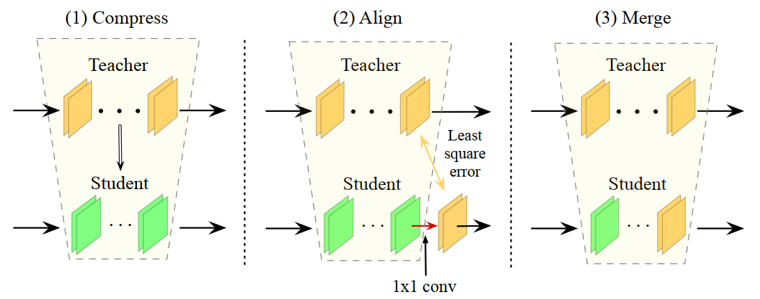
Figure 1: Three-step of few-sample knowledge distillation. (1) obtain student-net by compressing teacher-net; (2) add an 1×1 conv-layer at the end of each block of student-net, and align teacher and student by estimating the 1×1 conv-layer’s parameter using least-squared regression; (3) Merge the added 1× 1 conv-layer into the previous conv-layer to obtain final student-net. 

图1：少样本知识提取的三个步骤。（1） 通过压缩教师网络获取学生网络；（2） 在每个学生网络块的末端添加一个1×1 conv层，并通过使用最小二乘回归估计1×1 conv层的参数来对齐教师和学生；（3） 将添加的1×1 conv层合并到上一个conv层中，以获得最终的学生网络。

FSKD has many potential usages, especially when full fine-tuning or re-training is infeasible in practice, or the data at hand is only very limited. We name a few concrete cases below. First, edge devices have limited computing resources, while FSKD offers the possibility of on-device learning to compress deep models. Second, FSKD may help cloud services obtain a compact model when only a few unlabeled data is uploaded by the customer due to privacy or confidential issues. Third, FSKD enables fast model convergence if there is a strict time budget for training/fine-tuning. The strong practice requests have been addressed by several recent workshops .

FSKD有许多潜在用途，尤其是在实践中无法进行全面微调或重新训练，或者手头的数据非常有限的情况下。下面我们列举几个具体案例。首先，边缘设备的计算资源有限，而FSKD提供了在设备上学习压缩深度模型的可能性。其次，由于隐私或机密问题，当客户只上传了少量未标记的数据时，FSKD可以帮助云服务获得紧凑的模型。第三，如果有严格的训练/微调时间预算，FSKD可以实现快速模型收敛。最近的几次研讨会已经解决了强烈的实践要求。

Our major contributions can be summarized as follows:
• To the best of our knowledge, we are the first to show that accuracy recovery from a compressed network can be done with few unlabeled samples within minutes using knowledge distillation on desktop PC.
• Extensive experiments show that the proposed FSKD method is widely applicable to deep neural networks compressed by different pruning or decompositionbased methods.
• We demonstrate significant accuracy improvement from FSKD over existing distillation techniques, as well as compression-ratio and speedup gain over traditional pruning/decomposition-based methods on various datasets and network architectures

我们的主要贡献可以总结如下：
•据我们所知，我们率先证明，使用台式PC上的知识蒸馏，几分钟内就可以用少量未标记的样本从压缩网络中恢复准确度。
•大量实验表明，所提出的FSKD方法广泛适用于通过不同剪枝或基于分解的方法压缩的深层神经网络。
•我们证明，与现有蒸馏技术相比，FSKD的精确度有了显著提高，与基于各种数据集和网络架构的传统修剪/分解方法相比，压缩比和加速增益也有了显著提高

相关工作

Network Pruning methods obtain a small network by pruning weights from a trained larger network, which can keep the accuracy of the larger model if the prune ratio is set properly. [12] proposes to prune the individual weights that are near zero. Recently, filter pruning has become increasingly popular thanks to its better compatibility with off-the-shelf computing libraries, compared with weights pruning. Different criteria have been proposed to select the filters to be pruned, including norm of weights [24], scales of multiplicative coefficients [26], statistics of next layer [28], etc. These pruning based methods usually require iterative loop between pruning and fine-tuning for achieving better pruning ratio and speedup. Meanwhile, Network Decomposition methods try to factorize parameter-heavy layers into multiple lightweight ones. For instance, it may adopt low-rank decomposition to fully-connection layers [7], and different kinds of weight decomposition to convlayers [19, 20, 38]. However, aggressive network pruning or network decomposition usually lead to large accuracy drops, thus fine-tuning is a must to alleviate those drops [24, 26].

网络剪枝方法通过对训练后的大网络进行权值剪枝得到一个小网络，如果剪枝率设置得当，可以保持大模型的精度。[12] 建议删减接近零的单个权重。最近，与权重修剪相比，过滤器修剪由于与现成计算库更好的兼容性而变得越来越流行。人们提出了不同的标准来选择要修剪的过滤器，包括权重范数[24]、乘法系数的尺度[26]、下一层的统计[28]等。这些基于修剪的方法通常需要在修剪和微调之间进行迭代循环，以获得更好的修剪率和加速。同时，网络分解方法尝试将参数重层分解为多个轻层。例如，它可以对完全连接层[7]采用低秩分解，对连接层[19,20,38]采用不同类型的权重分解。然而，激进的网络修剪或网络分解通常会导致精度大幅下降，因此必须进行微调以缓解这些下降[24,26]。

Knowledge Distillation (KD) transfers knowledge from a pre-trained large teacher-net (or even an ensemble of networks) to a small student-net, for facilitating the deployment at test time. Originally, this is done by regressing the softmax output of the teacher model [15]. The soft continuous regression loss used here provides richer information than the label based loss, so that the distilled model can be more accurate than training on labeled data with cross-entropy loss. Later, various works have extended this approach by matching other statistics, including intermediate feature responses [32, 6], gradient [34], distribution [18], Gram matrix [37], etc. More complicatedly, deep mutual learning [39] trains a cohort of student-nets and teaches each other collaboratively with model distillation throughout the training process. The student-nets in KD are usually designed with random weight initialization, and thus all these methods require a large amount of data (known as the “transfer set”) to transfer the knowledge

知识提炼（KD）将知识从预先训练过的大型教师网络（甚至是网络集合）转移到小型学生网络，以便于在测试时部署。最初，这是通过回归教师模型的softmax输出来实现的[15]。与基于标签的损失相比，这里使用的软连续回归损失提供了更丰富的信息，因此提取的模型比基于交叉熵损失的标签数据的训练更准确。后来，各种工作通过匹配其他统计数据扩展了这种方法，包括中间特征响应[32,6]、梯度[34]、分布[18]、Gram矩阵[37]等。更复杂的是，深度相互学习[39]训练一组学生网络，并在整个训练过程中通过模型蒸馏相互协作。KD中的学生网络通常采用随机权重初始化设计，因此所有这些方法都需要大量数据（称为“转移集”）来转移知识

As a result, it is of great interest to start the studentnets with extremely pruned or decomposed networks and explore a KD solution under the few-sample setting. The proposed FSKD has a quite different philosophy on aligning intermediate responses to the closest knowledge distillation method FitNet [32]. FitNet re-trains the whole student-net with intermediate supervision as well as label supervision using a larger amount of fully-annotated data, while FSKD only estimates parameters of the added 1×1 conv-layer with few unlabeled samples. Experiments verify that FSKD is not only more efficient but also more accurate than FitNets

因此，我们非常感兴趣的是用经过修剪或分解的网络来启动学生网络，并在少样本设置下探索KD解决方案。拟议的FSKD在将中间响应与最接近的知识蒸馏方法FitNet[32]对齐方面有着完全不同的理念。FitNet通过中间监督和标签监督对整个学生网络进行了重新训练，使用了大量完全标注的数据，而FSKD仅估计添加的1×1 conv层的参数，几乎没有未标记的样本。实验证明，FSKD不仅比FitNets更有效，而且更准确

Learning with few samples has been extensively studied under the concept of one-shot or few-shot learning. One category of methods directly model few-shot samples with generative models [8, 23, 5, 3], while most others study the problem under the notion of transfer learning [2, 31]. In the latter category, meta-learning methods [35, 9] solve the problem in a learning-to-learn fashion, which has been recently gaining momentum due to their application versatility. Most studies are devoted to the image classification task, while it is still less-explored for knowledge distillation from few samples. Recently, some works tried to address this problem. [21] constructs pseudo-examples using the inducing point method and develops a complicated algorithm to optimize the model and pseudo-examples alternatively. [27] records per-layer meta-data for the teacher-net in order to reconstruct a training set, and then adopts a standard training procedure to obtain the student-net. Both are very costly due to the complicated and heavy training procedure. On the contrary, we aim for an efficient solution for knowledge distillation from few unlabeled samples.

在单样本或少样本学习的概念下，对少样本学习进行了广泛的研究。其中一类方法使用生成模型直接对少样本建模[8,23,5,3]，而大多数其他方法则在迁移学习的概念下研究该问题[2,31]。在后一类中，元学习方法[35,9]以一种从学习到学习的方式解决了这个问题，由于其应用的多功能性，这种方式最近得到了发展。大多数研究都致力于图像分类任务，而对于从少数样本中提取知识的研究则更少。最近，一些工作试图解决这个问题。[21]使用诱导点法构造伪示例，并开发一个复杂的算法来交替优化模型和伪示例。[27]记录教师网络的每层元数据，以重建训练集，然后采用标准训练程序获得学生网络。由于复杂而繁重的培训程序，这两种方法都非常昂贵。相反，我们的目标是从少数未标记的样本中有效地提取知识。

方法

3.1. Overview

Our FSKD method consists of three steps as shown in Figure 1. First, we obtain a student-net either by pruning or by decomposing the teacher-net. Second, we add a 1×1 conv-layer at the end of each block of the student-net and align the block-level outputs between teacher and student by estimating the parameters of the added layer from few unlabeled samples. Third, we merge the added 1×1 conv-layer into the previous conv-layer so that it will not introduce extra parameters and computation cost into the student-net

我们的FSKD方法由三个步骤组成，如图1所示。首先，我们通过剪枝或分解教师网络来获得学生网络。其次，我们在学生网络的每个块末端添加一个1×1 conv层，并通过从几个未标记的样本估计添加层的参数来对齐教师和学生之间的块级输出。第三，我们将添加的1×1 conv层合并到之前的conv层中，这样就不会在学生网络中引入额外的参数和计算成本。

Three reasons make the idea works efficiently. First, the compressed student-net inherits partial representation power from the teacher network, so adding 1×1 conv-layer is enough to calibrate the student-net and restore the accuracy. Second, the 1×1 conv-layers have relatively fewer parameters, which do not require too many data for the estimation. Third, the block-level output from teacher-net provides rich information as shown in FitNet [32]. Below, we will first describe our algorithm for block-level output alignment, and then prove why the added 1×1 conv-layer can be merged into the previous conv-layer. 

三个原因使这个想法有效地发挥作用。首先，压缩后的学生网络继承了教师网络的部分表示能力，因此添加1×1 conv层就足以校准学生网络并恢复准确性。第二，1×1 conv层的参数相对较少，估计时不需要太多数据。第三，教师网的模块级输出提供了丰富的信息，如FitNet[32]所示。下面，我们将首先描述块级输出对齐的算法，然后证明为什么添加的1×1 conv层可以合并到之前的conv层中。

3.2. Block-level Alignment

In this section, we provide details of our block-level output alignment algorithm. Suppose are the block-level output in matrix form for the student-net and teacher-net respectively, where d is the per-channel feature map resolution size. We add a 1×1 conv-layer Q at the end of each block of student-net before non-linear activation. As Q is degraded to the matrix form, it can be estimated with least squared regression as

在本节中，我们将详细介绍块级输出对齐算法。假设分别是学生网络和教师网络的矩阵形式的块级输出，其中d是每通道特征地图分辨率大小。在非线性激活之前，我们在每个学生网络块的末端添加一个1×1 conv层Q。当Q退化为矩阵形式时，可以用最小二乘回归估计为：

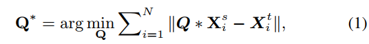
where N is the number of label-free samples used, and “*” means matrix product. The number of parameters of Q is, where no is the number of output channels in the block, which is usually not too large so that we can estimate Q with a limited number of samples.

其中N是使用的无标签样品数量，“*”表示矩阵积。Q的参数数是，其中no是块中的输出通道数，通常不会太大，因此我们可以在有限的样本数下估计Q。

Suppose there are M corresponding blocks in the teacher-net and the student-net required to align, to achieve our goal, we need minimize the following loss function 

假设教师网络和学生网络中有M个对应的块需要对齐，为了实现我们的目标，我们需要最小化以下损失函数 

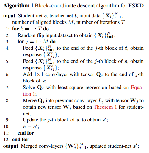
where Qj is the tensor for the added 1×1 conv-layer of the j-th block. In practice, we optimize this loss with a block-coordinate descent (BCD) algorithm [36], which greedily handles each of the M blocks in the student-net sequentially as shown in Algorithm-1 (FSKD-BCD). We can also minimize this loss using standard SGD on all added parameters (FSKD-SGD). However, FSKD-BCD has the following advantages over FSKD-SGD: (1) The BCD algorithm processes each block greedily with a sequential update rule, and each Q can be solved with the same set of few samples by aligning the block-level responses between teacher-net and student-net, while standard SGD considers {Qj} all together which theoretically requires more data. (2) The BCD algorithm is much more efficient, which can be usually done in less than a minute. 

式中，Qj是第j块增加的1×1 conv层的张量。在实践中，我们使用块坐标下降（BCD）算法[36]优化这种损失，该算法按顺序处理学生网络中的M个块，如算法1（FSKD-BCD）所示。我们还可以在所有附加参数（FSKD-SGD）上使用标准SGD将这种损失降至最低。然而，与FSKD-SGD相比，FSKD-BCD具有以下优点：（1）BCD算法使用顺序更新规则贪婪地处理每个块，通过对齐教师网和学生网之间的块级响应，每个Q可以用相同的少量样本集求解，而标准SGD考虑 {Qj}，理论上需要更多数据。（2） BCD算法效率更高，通常可以在不到一分钟内完成。

Unless otherwise noted, we use the FSKD-BCD algorithm with one iteration in our experiments. Appendix-A evaluates FSKD with more BCD iterations. Appendix-B makes a comparison between FSKD-BCD and FSKD-SGD.

除非另有说明，我们在实验中使用了一次迭代的FSKD-BCD算法。附录A使用更多BCD迭代来评估FSKD。附录B对FSKD-BCD和FSKD-SGD进行了比较。

3.3. Mergeable 1×1 conv-layer

Now we prove that the added 1x1 conv-layer can be merged into the previous conv-layer without introducing additional parameters and computation cost during inference.

现在，我们证明了添加的1x1 conv层可以合并到之前的conv层中，而无需在推理过程中引入额外的参数和计算成本。

Theorem 1. A pointwise convolution with tensor Q ∈ can be merged into the previous convolution layer with tensor W ∈ to obtain the merged tensor, where ◦ is merging operator and if the following conditions are satisfied.

定理1。张量Q∈的逐点卷积可以与张量W∈合并到前一个卷积层中，得到合并张量,其中◦ 如果满足以下条件，则为合并算子和。

c1. The output channel number of W equals to the input channel number of Q, i.e., no = n0 i.
c2. No non-linear activation layer like ReLU [30] between W and Q. 

c1  W的输出通道数等于Q的输入通道数，即no=N0I。
c2  在W和Q之间没有像ReLU[30]那样的非线性激活层。 

The pointwise convolution can be viewed as a linear combination of the kernels in the previous convolution layer. Due to the space limitation, we put the formal proof and the detailed form of the merging operator in AppendixC. The number of output channels of W’ is n’o, which is different from that of W (i.e., no). It is easy to have the following corollary. 

逐点卷积可以看作是前一个卷积层中核的线性组合。由于篇幅的限制，我们在附录C中给出了合并算子的形式证明和详细形式。W’的输出通道数为n’o，这与W的输出通道数不同（即no）。很容易得出以下推论。

Corollary 1. When the following condition is satisfied,

c3. the number of input and output channels of Q equals to the number of output channel of W, i.e., ,

the merged convolution tensor W' has the same parameters and computation cost as W, i.e. both W' , W ∈ .

推论1   当满足下列条件时，

c3    Q的输入和输出通道数等于W的输出通道数，即

合并卷积张量W'的参数和计算量与W相同，即都是W ∈

This condition is required not only for ensuring the same parameter size and computing cost, but also for ensuring the output-size of current layer matching to the input-size of next layer so that these two layers are connectable.

这个条件不仅是为了确保参数大小和计算成本相同，而且是为了确保当前层的输出大小与下一层的输入大小匹配，以便这两层是可连接的。 

实验

We perform extensive experiments on different image classification datasets to verify the effectiveness of FSKD on various student-net construction methods and its advantages over existing distillation methods in terms of both accuracy and speed. Student-nets can be obtained either by pruning based methods such as filter pruning [24] and network slimming [26], or by decomposition-based methods such as network decoupling [10]. We implement the code with PyTorch, and conduct experiments on a desktop PC with Intel i7-7700K CPU and one NVidia 1080TI GPU. The code will be made publicly available. For all experiments, the results are averaged over 5 trials of different randomly selected images.

我们在不同的图像分类数据集上进行了大量实验，以验证FSKD在各种学生网络构建方法上的有效性，以及它在准确性和速度方面优于现有的提取方法。学生网络可以通过基于剪枝的方法获得，比如过滤器剪枝[24]和网络瘦身[26]，或者通过基于分解的方法获得，比如网络解耦[10]。我们用Pytorh实现了该代码，并在一台带有Intel i7-7700K CPU和一个NVidia 1080TI GPU的台式PC上进行了实验。该准则将公开发布。对于所有的实验，结果都是对随机选择的不同图像进行5次试验的平均值。

4.1. Student-net from Pruning teacher-net

Filter Pruning

We first obtain the student-nets using the filter pruning method [24], which prunes out conv-filters according to the L1 norm of their weights. The L1 norm of filter weights are sorted and the smallest portion of filters will be pruned to reduce the number of filter-channels in a conv-layer. Figure 2 illustrates how FSKD works for block-level alignment in this case. Note that the number of channels in teacher-net may be different from that in student-net. However, we only match the un-pruned part of feature-maps in teacher-net to the feature maps in the student-net so that FSKD is applicable in this case.

我们首先使用过滤器修剪方法[24]获得学生网络，该方法根据conv过滤器权重的L1范数修剪conv过滤器。对滤波器权重的L1范数进行排序，并对滤波器的最小部分进行修剪，以减少conv层中的滤波器通道数。图2说明了在这种情况下，FSKD如何用于块级对齐。请注意，教师网络中的频道数量可能与学生网络中的频道数量不同。然而，我们只将教师网络中未删减的部分特征映射匹配到学生网络中的特征映射，因此FSKD适用于这种情况。

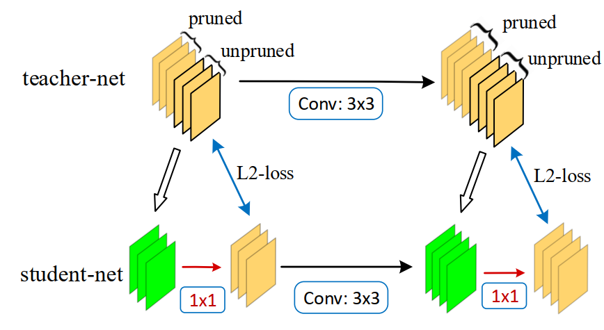
Figure 2: Illustration of FSKD on filter pruning and network slimming. At each block, we copy weights of the unpruned part in teacher-net to student-net, and align the feature maps of studentnet to those unpruned feature maps of teacher-net by adding a 1×1 conv-layer (red-color) with L2-loss. The added 1×1 layer can be merged into the previous conv-layer in student-net.
图2:FSKD关于过滤器修剪和网络缩减的说明。在每个区块，我们将教师网络中未运行部分的权重复制到学生网络，并通过添加一个1×1 conv层（红色）和L2损失，将学生网络的特征映射与教师网络中未运行的特征映射对齐。添加的1×1层可以合并到学生网的前一个conv层中。

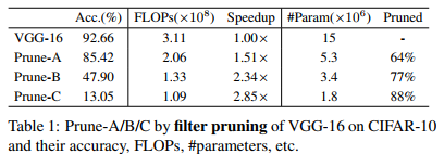
We make a comprehensive study of VGG-16 [33] on CIFAR-10 dataset to evaluate the performance of FSKD along with three different pruning settings. First, we follow the original pruning scheme of [24] and obtain PruneA. Second, we propose another more aggressive pruning scheme named Prune-B, which prunes 10% more filters in the aforementioned layers, and also pruned 20% filters for the remaining layers. Third, since previous works show that one time extremely pruning may yield the pruned network unable to recovery from fine-tuning, while the iteratively pruning and fine-tuning procedure is observed effective to obtain extreme model compression [11, 24, 26], we propose Prune-C which iteratively runs the pruning and FSKD procedure as described in Appendix-D for 2 iterations to achieve higher compression rate. Table 1 lists the accuracy, FLOPs and #parameter information for three student-nets obtained by these pruning schemes.

我们在CIFAR-10数据集上对VGG-16[33]进行了全面研究，以评估FSKD的性能以及三种不同的修剪设置。首先，我们遵循[24]的原始修剪方案，得到PruneA。其次，我们提出了另一种更具攻击性的剪枝方案Prune-B，该方案在上述层中剪枝10%以上的过滤器，并在其余层中剪枝20%的过滤器。第三，由于之前的工作表明，一次极端修剪可能会导致修剪后的网络无法从微调中恢复，而迭代修剪和微调过程可以有效地获得极端模型压缩[11,24,26]，我们提出了Prune-C，它迭代运行附录D中描述的修剪和FSKD过程，进行2次迭代，以获得更高的压缩率。表1列出了通过这些修剪方案获得的三个学生网络的精度、FLOPs和#参数信息。 

For the few-sample setting, we randomly select 100 (10 for each category) and 500 (50 for each category) images from the CIFAR-10 training set, and keep them fixed in all experiments. We evaluate 5 different randomly-selected image set and report the mean and std of accuracy. Table 2 lists the results of different methods of recovering a pruned network, including FitNet [32], fine-tuning with limited data and full training data [24]. 

对于少数样本设置，我们从CIFAR-10训练集中随机选择100（每个类别10个）和500（每个类别50个）图像，并在所有实验中保持固定。我们评估了5种不同的随机选择的图像集，并报告了准确性的平均值和标准差。表2列出了恢复修剪网络的不同方法的结果，包括FitNet[32]、使用有限数据进行微调和完整训练数据[24]。

As shown in Table 2, our method is much more efficient and provides better accuracy recovery than both FitNet and the fine-tuning procedure adopted in [24], and also more robust with a different set of selected images. For instance, for Prune-B with only 500 samples, our method can recover the accuracy from 47.9% to 91.2% in 19.3s, while FitNet has to take 157.1s to recover the accuracy to 90.7%, and fewsample fine-tuning can only recover the accuracy to 83.4%. When full training set available, it takes about 30 minutes for full fine-tuning to reach similar accuracy as FSKD. This demonstrates the big advantages of FSKD over full finetuning based solutions.

如表2所示，与FitNet和[24]中采用的微调程序相比，我们的方法效率更高，提供了更好的精度恢复，并且对于不同的选定图像集也更稳健。例如，对于只有500个样本的Prune-B，我们的方法可以在19.3秒内将准确度从47.9%恢复到91.2%，而FitNet需要157.1秒才能将准确度恢复到90.7%，而fewsample微调只能将准确度恢复到83.4%。当完整的训练集可用时，完全微调需要大约30分钟才能达到与FSKD类似的精度。这证明了FSKD相对于基于全微调的解决方案的巨大优势。

 

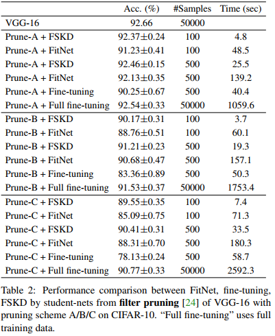
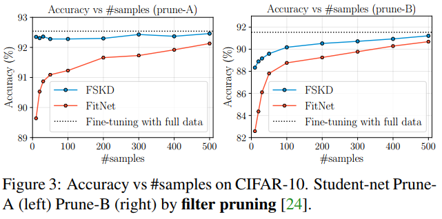
Figure 3 further studies the performance versus different amount of training samples. Our method keeps outperforming FitNet under the same training samples. In particular, FitNet experiences a noticeable accuracy drop when the number of samples is less than 100, while FSKD can still recover the accuracy of the pruned network to a high level 

图3进一步研究了不同训练样本量下的性能。在相同的训练样本下，我们的方法始终优于FitNet。特别是，当样本数小于100时，FitNet的准确度会显著下降，而FSKD仍然可以将修剪后的网络的准确度恢复到较高水平

 We further illustrate the per-layer (block) feature responses difference between teacher-net and student-net before and after using FSKD in Figure 4a. Before applying FSKD, the correlation between teacher-net and student-net is broken due to aggressive compression. However, after FSKD, the per-layer correlations are mostly restored. This verifies the ability of FSKD for recovering lost information. We also show the accuracy change during sequentially block-level alignment in Figure 4b, which clearly demonstrate the effectiveness of our sequentially block-by-block update in the FSKD algorithm. 

在图4a中，我们进一步说明了使用FSKD前后教师网络和学生网络的每层（块）特征响应差异。在应用FSKD之前，教师网络和学生网络之间的相关性由于积极的压缩而被打破。然而，在FSKD之后，每层的相关性基本恢复。这验证了FSKD恢复丢失信息的能力。我们还在图4b中显示了顺序块级对齐过程中的精度变化，这清楚地证明了我们在FSKD算法中顺序逐块更新的有效性。

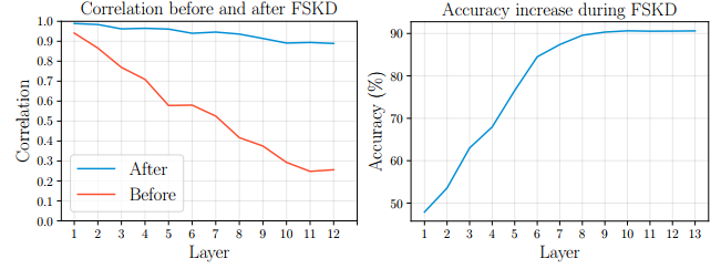
Figure 4: Left: Layer-level output correlation between teacher-net and student-net before and after FSKD on student-nets (Prune-A) by filter pruning [24]. Right: Accuracy change during sequentially block-level alignment.
图4：左图：通过过滤器修剪，在学生网络上进行FSKD前后，教师网络和学生网络之间的层级输出相关性（Prune-A）[24]。右图：连续块级对齐期间的精度变化。 

Network Slimming

We then study the student-net from another filter pruning method named network slimming [26], which removes insignificant filter channels and corresponding feature maps using sparsified channel scaling factors. Network slimming consists of three steps: sparse regularized training, pruning and fine-tuning. Here, we replace the time-consuming finetuning step with our FSKD, and follow the original paper [26] to conduct experiments to prune different networks on different datasets. The alignment framework is the same as the filter pruning case as shown in Figure 2.

然后，我们从另一种名为“网络缩减”的过滤器修剪方法[26]中研究学生网络，该方法使用稀疏的通道比例因子去除不重要的过滤器通道和相应的特征映射。网络瘦身包括三个步骤：稀疏正则化训练、修剪和微调。在这里，我们用我们的FSKD取代了耗时的微调步骤，并按照原始论文[26]进行实验，在不同的数据集上修剪不同的网络。对齐框架与过滤器修剪情况相同，如图2所示。

We apply FSKD on networks pruned from VGG-19, ResNet-164, and DenseNet-40 [17], on both CIFAR-10 and CIFAR-100 datasets. Table 3 lists results on CIFAR-10, while Table 4 lists results on CIFAR-100. Note that the filter-prune-ratio (like 70% in Table 3) means the portion of filters that are removed in comparison to the total number of filters in the network. We also apply FSKD on networks pruned from VGG-A (or VGG-11) on ImageNet dataset, as shown in Table 5.

我们将FSKD应用于从VGG-19、ResNet-164和DenseNet-40[17]中删减的网络，同时应用于CIFAR-10和CIFAR-100数据集。表3列出了CIFAR-10的结果，而表4列出了CIFAR-100的结果。请注意，过滤器删减率（如表3中的70%）是指与网络中过滤器总数相比被删除的过滤器部分。我们还将FSKD应用于从ImageNet数据集上的VGG-A（或VGG-11）修剪的网络，如表5所示。

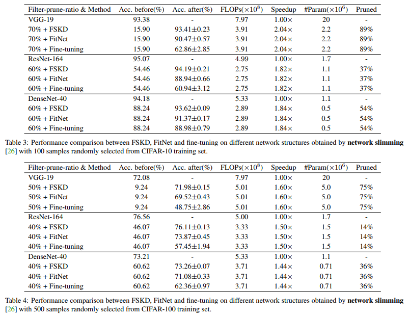
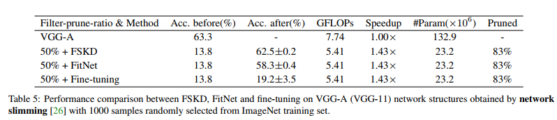The results show that that FSKD consistently outperforms FitNet and fine-tuning with a notable margin under the few-sample setting on all evaluated networks and datasets. This study demonstrates that FSKD is universally applicable to various network structure and pruning methods, and can recover the accuracy of the pruned network using few unlabeled samples to the same level of fine-tuning using fully annotated training dataset.

结果表明，在所有评估的网络和数据集上，FSKD始终优于FitNet和微调，在少样本设置下具有显著的优势。这项研究表明，FSKD普遍适用于各种网络结构和修剪方法，并且可以使用少量未标记样本将修剪后的网络的精度恢复到使用完全注释的训练数据集进行微调的相同水平。

4.2. Student-net from Decomposing teacher-net

In this section, we apply FSKD on a decompositionbased method called network decoupling [10], which can decompose a regular convolution layer into the sum of several depth-wise separable blocks, where each such block consists of a depth-wise (DW) conv-layer and a point-wise (PW, 1×1) conv-layer. The compression ratio increases as the number (T ) of such blocks decreases, but the accuracy of the compressed model will also drop. Since each decoupled block ends with a 1×1 convolution, we can apply FSKD at the end of each decoupled block. Figure 5 illustrates how FSKD works for block-level alignment in this case.

在本节中，我们将FSKD应用于一种基于分解的方法，称为网络解耦[10]，该方法可以将规则卷积层分解为几个深度可分离块的总和，其中每个这样的块由一个深度（DW）conv层和一个点（PW，1×1）conv层组成。压缩比随着此类块的数量（T）的减少而增加，但压缩模型的精度也会下降。由于每个解耦块以1×1卷积结束，我们可以在每个解耦块的末尾应用FSKD。图5说明了在这种情况下，FSKD如何用于块级对齐。

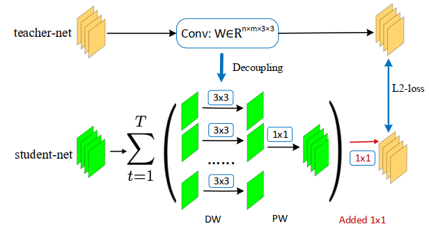
 Figure 5: Illustration of FSKD on network decoupling. At each block of teacher-net, we decouple regular-conv into a sum of depthwise + pointwise conv-layers as the block of student-net, and align the feature maps of student-net to that of teacher-net by adding a 1×1 conv-layer (red-color) with L2-loss. The added layer can be merged into previous the pointwise layer in student-net.

图5：网络解耦的FSKD示意图。在教师网络的每个区块，我们将常规conv解耦为深度+点方向的conv层之和，作为学生网络的区块，并通过添加1×1 conv层（红色）和L2损失，将学生网络的特征映射与教师网络的特征映射对齐。添加的层可以合并到学生网络中的前一个逐点层中。

Following [10], we obtain student-nets by decoupling VGG-16 and ResNet-18 pre-trained on ImageNet with different T values. We evaluate the resulted network performance on the validation set of the ImageNet classification task. We randomly select one image from each of the 1000 classes in ImageNet training set to obtain 1000 samples as our FSKD training set. Table 6 shows the top-1 accuracy of student-net before and after applying FSKD on VGG-16 and ResNet-18.

在[10]之后，我们通过解耦VGG-16和ResNet-18在ImageNet上以不同的T值预先训练来获得学生网络。我们在ImageNet分类任务的验证集上评估结果网络性能。我们从ImageNet训练集中的1000个类中随机选择一幅图像，以获得1000个样本作为我们的FSKD训练集。表6显示了在VGG-16和ResNet-18上应用FSKD前后，学生网络的最高精确度。

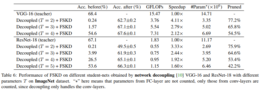
It is quite interesting to see that when T is small, we can recover the accuracy of student-net from nearly random guess (0.24%, 0.21%) to a much higher level (62.7% and 49.5%) with only 1000 samples. One possible explanation is that the highly-compressed networks still inherit some representation power from the teacher-net i.e., the depth-wise 3×3 convolution, while lacking the ability to output meaningful predictions due to the degraded and inaccurate 1×1 convolution. The FSKD calibrates the 1×1 convolution by aligning the block-level responses between teacher-net and student-net so that the lost information in 1×1 convolution is compensated, and reasonable recovery is achieved.

有趣的是，当T很小时，我们可以用1000个样本将学生网络的准确度从几乎随机的猜测（0.24%，0.21%）恢复到更高的水平（62.7%和49.5%）。一种可能的解释是，高度压缩的网络仍然从教师网络继承了一些表示能力，即深度方向的3×3卷积，但由于1×1卷积的退化和不准确，因此缺乏输出有意义预测的能力。FSKD通过对齐教师网和学生网之间的块级响应来校准1×1卷积，从而补偿1×1卷积中丢失的信息，并实现合理的恢复。

In all the other cases, FSKD can recover the accuracy of a highly-compressed network to be comparable with the original network. This shows that FSKD can be applied to student-net compressed by network decomposition, and that FSKD can achieve great performance on large and difficult dataset such as ImageNet

在所有其他情况下，FSKD可以恢复高度压缩网络的精度，使其与原始网络相当。这表明，FSKD可以应用于通过网络分解压缩的学生网络，并且FSKD可以在ImageNet等大型和困难的数据集上实现良好的性能

分析与讨论

FSKD with Arbitrary Data

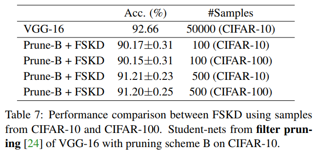
In this section, we try to answer the following question: is FSKD totally label-free? For example, is FSKD still valid if the available few samples are arbitrary images and the teacher network never sees these images before? To answer this question, we evaluate FSKD’s performance on VGG-16 model trained on CIFAR-10 and compressed using filter pruning (prune-B), with the few samples for FSKD are randomly selected from CIFAR-100 instead of CIFAR-10

在本节中，我们试图回答以下问题：FSKD是否完全没有标签？例如，如果可用的少数样本是任意图像，并且教师网络以前从未见过这些图像，那么FSKD仍然有效吗？为了回答这个问题，我们评估了FSKD在基于CIFAR-10训练的VGG-16模型上的性能，并使用过滤器修剪（prune-B）进行压缩，FSKD的少量样本是从CIFAR-100而不是CIFAR-10中随机选择的

As shown in Table 7, there is no statistical difference in accuracy between FSKD using data from CIFAR-10 or CIFAR-100. This shows that FSKD aligns the student-net with the teacher-net without any information about the labels of the data. Even if the input images are of classes it has never seen before (CIFAR-100 does not include classes in CIFAR-10), FSKD can still recover the student network to the same accuracy level. This further demonstrates FSKD’s potential in situations where only a few samples of unlabeled data are available

如表7所示，使用CIFAR-10或CIFAR-100数据的FSKD在准确性上没有统计学差异。这表明FSKD将学生网络与教师网络对齐，而不提供任何有关数据标签的信息。即使输入图像是以前从未见过的类（CIFAR-100不包括CIFAR-10中的类），FSKD仍然可以将学生网络恢复到相同的精度水平。这进一步证明了FSKD在只有少量未标记数据样本可用的情况下的潜力

 What if student-nets are hand-designed?

Our previous experiments construct student-nets by pruning or decomposing teacher-net, and then apply FSKD to boost their performance. People may be interested in the problem “what if student-nets are hand-designed with random initialization”. In fact, there are two existing works [21, 27] making some pioneer trials on this topic with specific methods for “pseudo” examples generation. Here we conduct experiments to compare our method to these two methods under the same few-sample setting on the same dataset MNIST, for a fair comparison.

我们之前的实验通过修剪或分解教师网络来构建学生网络，然后应用FSKD来提高其性能。人们可能会对这个问题感兴趣，“如果学生网络是用随机初始化手工设计的呢？”。事实上，已有两个工作[21,27]对这一主题进行了一些开创性的尝试，并给出了生成“伪”示例的具体方法。在这里，我们在相同的数据集MNIST上进行实验，在相同的少数样本设置下，将我们的方法与这两种方法进行比较，以进行公平的比较。

Due to different network structures used in these two methods, we make a separate comparison. For [21], the teacher-net has 3 conv-layers followed by 2 fully-connected layers. For [27], the teacher-net is a standard LeNet-5. For both cases, the student-net is the “half-sized” to that of the corresponding teacher-net in terms of the number of feature map channels per conv-layers. As the channel number between student-net and teacher-net is different, we adopt the same strategy as in Figure 2 for filter pruning. That means, the student-net only corresponds to the un-pruned part of the teacher-net, which is obtained the same as [24]. One difference is that we did not copy the weight from un-pruned part of teacher-net to the student-net, while keeping the weight of student-net randomly initialized. For both cases, we compared our FSKD with (1) standard SGD trained on few samples with labeled loss; (2) method from [21] or [27] under the same setting; (3) the FitNet method trained on few samples. In order to better simulate the few-sample setting, we do not apply data augmentation to the training set. We randomly pick 10, 20, 50, 100 and 200 samples from the MNIST training set and keep these few-sample sets fixed across this study. Table 8 lists the comparison results. It shows that SGD with few samples performs the worst, while [21] performs better on the same settings than SGD (still worse in the case of 200 samples). The data-free method [27] performs better than SGD. On both cases, FitNet shows much better performance than SGD and the two compared methods, while our FSKD further outperform FitNet with a noticeable gap, where the gap becomes smaller and smaller when the number of samples increases. This may be due to the following reason. FSKD can be viewed as a special case of FitNet. FitNet optimizes all the weights between teachernet and student-net using standard SGD algorithm, while FSKD optimizes only the weights from added 1×1 convlayers in student-net with the BCD algorithm. The BCD algorithm is more sample-efficient than the SGD based algorithm so that FSKD performs both much more efficient and accurate than FitNet on few-sample settings. When training samples used are increased, FSKD will converge to FitNet in the end

由于这两种方法使用的网络结构不同，我们将分别进行比较。对于[21]，教师网有3个conv层，后面是2个完全连接的层。对于[27]，教师网是标准的LeNet-5。对于这两种情况，就每个conv层的特征映射通道数量而言，学生网络的“大小”是相应教师网络的“一半”。由于学生网和教师网之间的通道数不同，我们采用与图2相同的策略进行过滤器修剪。这意味着，学生网只对应于教师网的未删减部分，其获得方式与[24]相同。一个区别是，我们没有将未修剪部分的教师网络的权重复制到学生网络，同时保持学生网络的权重随机初始化。对于这两种情况，我们将我们的FSKD与（1）标准SGD进行了比较，标准SGD只针对少数标记丢失的样本进行训练；（2） [21]或[27]中相同设置下的方法；（3） FitNet方法只对少数样本进行了训练。为了更好地模拟较少的样本设置，我们不对训练集应用数据扩充。我们从MNIST训练集中随机选取10、20、50、100和200个样本，并在整个研究中固定这几个样本集。表8列出了比较结果。结果表明，样本数较少的SGD性能最差，而[21]在相同设置下的性能优于SGD（在样本数为200的情况下更差）。无数据方法[27]的性能优于SGD。在这两种情况下，FitNet的性能都比SGD和两种比较方法好得多，而我们的FSKD进一步优于FitNet，存在明显的差距，随着样本数量的增加，差距越来越小。这可能是由于以下原因。FSKD可视为FitNet的特例。FitNet使用标准SGD算法优化教师网和学生网之间的所有权重，而FSKD仅使用BCD算法优化学生网中添加的1×1层的权重。与基于SGD的算法相比，BCD算法的采样效率更高，因此FSKD在较少的采样设置下比FitNet执行的效率和精度都要高得多。当使用的训练样本增加时，FSKD最终将收敛到FitNet

结论

We proposed a novel yet simple method, namely fewsample knowledge distillation (FSKD) for efficient network compression, while “efficient” lies in both training/processing efficiency and label-free sample efficiency. FSKD works for student-nets constructed by either pruning or decomposing teacher-nets with different methods. It demonstrates great efficiency over fine-tuning based solution and advantages over traditional knowledge distillation methods like FitNet by a large margin in the few-sample setting, with extra merits that FSKD is totally label-free in the optimization.

我们提出了一种新颖而简单的方法，即有限样本知识提取（FSKD）来实现有效的网络压缩，而“有效”在于训练/处理效率和无标签样本效率。FSKD适用于通过使用不同方法修剪或分解教师网络而构建的学生网络。与基于微调的解决方案相比，该方法具有更高的效率，在较少的样本设置下，与FitNet等传统知识提取方法相比，该方法具有更大的优势，此外，FSKD在优化过程中完全没有标签。

附录

A: FSKD with different # BCD iterations

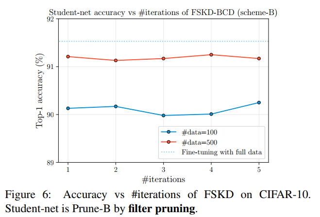
In our FSKD algorithm, we can apply the blockcoordinate descent for several iterations. However, we do not observe noticeable gains for the iteration number T > 1 over T = 1 as shown in Figure 6, so that we set T = 1 in all our following experiments. This may be due to the reason that in each iteration, the sub-problem is a linear optimization problem so that we can find exact minimization, which is consistent with the finding by [16].

在我们的FSKD算法中，我们可以应用块坐标下降进行多次迭代。然而，如图6所示，我们没有观察到迭代次数T>1对T=1的显著增益，因此我们在接下来的所有实验中都设置了T=1。这可能是因为在每次迭代中，子问题是一个线性优化问题，因此我们可以找到精确的最小化，这与[16]的发现一致。 

B: FSKD-BCD vs. FSKD-SGD

In this section, we compared two FSKD optimization algorithms: FSKD-BCD uses the BCD algorithm on blocklevel and FSKD-SGD optimizes the loss all together with the standard SGD algorithm. We valuate both methods on VGG-16 models trained on CIFAR-10 and compressed using filter pruning (prune-B). As shown in Table 9, FSKDBCD achieves better accuracy than FSKD-SGD while significantly improves time efficiency

在本节中，我们比较了两种FSKD优化算法：FSKD-BCD在块级使用BCD算法，FSKD-SGD与标准SGD算法一起优化损耗。我们在CIFAR-10上训练的VGG-16模型上评估了这两种方法，并使用过滤器修剪（prune-B）进行了压缩。如表9所示，FSKDBCD比FSKD-SGD具有更好的精度，同时显著提高了时间效率。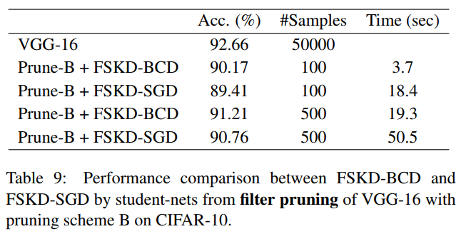

C: Proof of Theorem 1

Proof. When W is a point-wise convolution with tensor, both W and Q are degraded into matrix form. It is obvious that when condition c1 ∼ c3 satisfied, the theorem holds with W in this case, where ∗indicates matrix multiplication.

证据  当W是张量为的逐点卷积时，W和Q都退化为矩阵形式。显然，当条件c1∼c3 如果满足，则该定理在时成立。其中∗表示矩阵乘法。 

When W is a regular convolution with tensor W∈ , the proof is non-trivial. Fortunately, recent work on network decoupling [10] presents an important theoretic result as the basis of our derivation.

当W是张量为 W∈的正则卷积时，证明是非平凡的。幸运的是，最近关于网络解耦的研究[10]给出了一个重要的理论结果，作为我们推导的基础。 

Lemma 1. Regular convolution can be exactly expanded to a sum of several depth-wise separable convolutions. Formally, , where Pk ∈,

引理1。正则卷积可以精确地扩展为几个深度可分离卷积的和。形式上，，其中Pk ∈

where ◦ is the compound operation, which means performing Dk before Pk. 

其中◦ 是复合运算，即在Pk之前执行Dk。 

Please refer to [10] for the details of proof for this Lemma. When W is applied to an input patch x ∈ , we obtain a response vector y ∈ as

关于这个引理的详细证明，请参考[10]。当W应用于输入面片x∈时，我们得到一个响应向量y∈ as

 

where , and ⊗ here means convolution operation. is a tensor slice along the i-th input and o-th output channels, xi = x[i， :， :] is a tensor slice along the i-th channel of 3D tensor x. 

其中，以及⊗ 这里指的是卷积运算是沿第i个输入和第o个输出通道的张量切片，xi = x[i， :， :] 是沿三维张量x的第i个通道的张量切片。 

When point-wise convolution Q is added after Q without non-linear activation between them, we have 

当逐点卷积Q加在Q之后，它们之间没有非线性激活时，我们得到

 

With Lemma-1, we have 

 

As both Q and Pk are degraded into matrix form, denoting , we have .This proves the case when W is a regular convolution. 

因为Q和Pk都退化为矩阵形式，表示，我们有。这证明了W是正则卷积的情况。

D: Algorithm for iterative pruning and FSKD

Algorithm-2 describes the iteratively pruning and FSKD procedure to achieve extremely compression rate based on [11, 24, 26].

算法2描述了迭代剪枝和FSKD过程，以实现基于[11,24,26]的极高压缩率。 

E: Training only PW conv-layer is enough

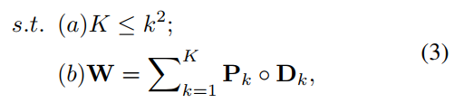
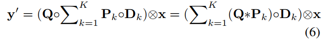
People may challenge that learning 1 × 1-conv may loss representation power and ask why the added 1 × 1 convolution works so well with such few samples. According to the network decoupling theory (Lemma-1), any regular convlayer could be decomposed into a sum of depthwise separable blocks, where each depthwise separable block consists of a depthwise (DW) convolution (for spatial correlation modeling) followed by a pointwise (PW) convolution (for cross-channel correlation modeling). The added 1 × 1 conv-layer is absorbed/merged into the previous PW layer finally. The decoupling yields that the number of parameters in PW-layer occupies most (>=80%) parameters of the whole network. We argue that learning only 1 × 1-conv is still very powerful, and make a bold hypothesis that PW conv-layer is more critical for performance than DW convlayer. To verify this hypothesis, we conduct experiments on VGG16 and ResNet50 on CIFAR-10 and CIFAR-100 under below different settings.

人们可能会质疑，学习1×1-conv可能会失去表征能力，并会问，为什么添加的1×1卷积在如此少的样本中工作得如此好。根据网络解耦理论（Lemma-1），任何规则层都可以分解为深度可分离块的总和，其中每个深度可分离块由深度（DW）卷积（用于空间相关建模）和点（PW）卷积（用于交叉信道相关建模）组成。添加的1×1 conv层最终被吸收/合并到之前的PW层中。解耦结果表明，PW层中的参数数量占整个网络的大部分（>=80%）。我们认为仅学习1×1-conv仍然非常有效，并大胆假设PW-conv层比DW-conv层对性能更为关键。为了验证这一假设，我们在以下不同设置下对CIFAR-10和CIFAR-100上的VGG16和ResNet50进行了实验。

(1) We train the network from random initialization with 160 epochs with learning-rate decay 1/10 at 80, 120 epochs from 0.01 to 0.0001. 
(2) We start from a random initialized network (VGG16 or ResNet50), and do full rank decoupling (K = k2 in Eq. 3) so that channels in DW layers are orthogonal, and PW layers are still fully random. Note that Lemma-1 ensures the network before and after decoupling are equivalent (i.e., able to transfer back and force from each other). We keep all the DW-layers fixed (with orthogonal basis from random data), and train only the PW layers with 160 epochs. We denote this scheme as ND-1*1.

（1） 我们对网络进行训练，从随机初始化到160个阶段，80个阶段学习率衰减1/10，120个阶段从0.01到0.0001。
（2） 我们从一个随机初始化的网络（VGG16或ResNet50）开始，进行满秩解耦（等式3中的K=k2），这样DW层中的信道是正交的，PW层仍然是完全随机的。请注意，Lemma-1确保解耦前后的网络是等效的（即，能够相互转换和施加力）。我们将所有DW层保持固定（使用随机数据的正交基），只训练具有160个历元的PW层。我们将这个方案表示为ND-1*1。

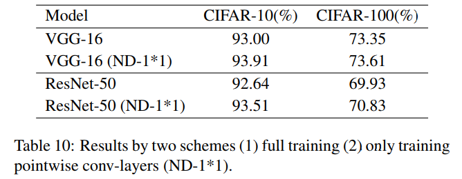
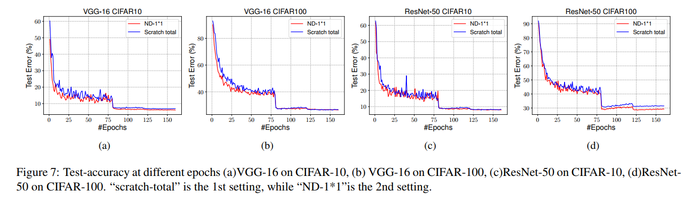
Note that except the setting explicitly described, all the other configurations (including training epochs, hyperparameters, hardware platform, etc) are kept the same on both experimental cases. Table 10 lists the experimental results on these two cases on both datasets with two different network structures. It is obvious that the 2nd case (ND-1*1) clearly outperforms the 1st case. Figure 7 further illustrates the test accuracy at different training epochs, which clear shows that the 2nd case (ND-1*1) converges faster and better than the 1st case. This experiment verifies our hypothesis that when keeping DW channels orthogonal, training only the pointwise (1×1) conv-layer is accurate enough, or even better than training all the parameters together.

请注意，除了明确描述的设置外，所有其他配置（包括训练时间、超参数、硬件平台等）在两个实验案例中都保持相同。表10列出了这两种情况下，在两种不同网络结构的数据集上的实验结果。显然，第二种情况（ND-1*1）明显优于第一种情况。图7进一步说明了不同训练时期的测试精度，这清楚地表明第二种情况（ND-1*1）比第一种情况收敛得更快、更好。本实验验证了我们的假设，即在保持DW通道正交的情况下，仅训练逐点（1×1）conv层是足够准确的，甚至比同时训练所有参数更好。

 

F: Filter Visualization

In this section, we try to answer why FSKD works so well that it can provide almost the same results as that of fine-tuning with full training set. We conduct experiments based on VGG-13 on CIFAR-10. For a given VGG-13 network, We first decouple a conv-layer to obtain one DW conv-layer and one PW conv-layer, as is done in network decoupling [10]. Then we visualize the PW conv-layer of the decoupled layer. For simplicity, we only visualize the PW conv-layer of the first decoupled layer. We do the visualization on three VGG-13 network with different parameters:

在本节中，我们试图回答为什么FSKD工作得如此之好，以至于它可以提供与使用完整训练集进行微调几乎相同的结果。我们在CIFAR-10上进行了基于VGG-13的实验。对于给定的VGG-13网络，我们首先解耦一个conv层，以获得一个DW conv层和一个PW conv层，如网络解耦[10]中所述。然后我们将分离层的PW conv层可视化。为简单起见，我们仅将第一个解耦层的PW conv层可视化。我们在三个具有不同参数的VGG-13网络上进行可视化：

(1) Initialize the VGG-13 network with the MSRA initialization (Figure 8 left).
(2) Run SGD based fine-tuning on 500 samples for VGG-13 with random initialization until convergence (Figure 8 middle).
(3) Run FSKD on 500 samples for VGG-13 with SGD based initialization (Figure 8 right). The teacher network is also a VGG-13 trained on full CIFAR-10 training set.

（1） 用MSRA初始化来初始化VGG-13网络（图8左）。
（2） 在VGG-13的500个样本上运行基于SGD的微调，并进行随机初始化，直到收敛（图8）。
（3） 使用基于SGD的初始化在VGG-13的500个样本上运行FSKD（图8右侧）。教师网络也是在完整的CIFAR-10训练集上训练的VGG-13。

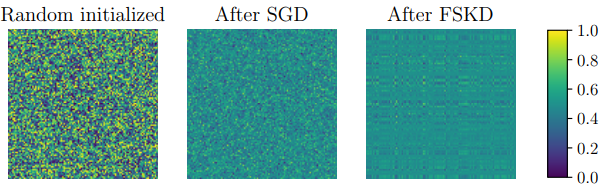
Figure 8: Decouple VGG-13 into DW conv-layer and PW convlayers, and show one PW conv-layer with random initialization (left), after SGD based fine-tuning (middle), and after FSKD (right). Note values of the PW tensor are scaled into the range (0,1.0) by the min/max values of the tensor for better visualization.
图8：将VGG-13解耦为DW conv层和PW conv层，并显示一个随机初始化的PW conv层（左）、基于SGD的微调后（中）和FSKD后（右）。注：PW张量的值通过张量的最小值/最大值缩放到范围（0,1.0）内，以便更好地可视化。 

It clearly shows that the PW conv-layer before fine-tuning is fairly random on the value range, the one after fine-tuning is less random, while the one after FSKD further starts to show some regular patterns, which demonstrates that FSKD can distill the knowledge from the teacher-net to student-net effectively with few samples. 

这清楚地表明，微调前的PW conv层在值范围上是相当随机的，微调后的PW conv层的随机性较小，而FSKD后的PW conv层进一步开始显示出一些规律性，这表明FSKD可以用较少的样本有效地将知识从教师网络提取到学生网络。