Kaggle Predict Future Sales interpretions

1.data explanation

1.1item_categories

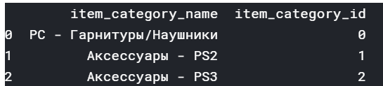
item_categories contains two attributes
item_category_name and item_category_id
1.2

items contain 3 attributes item_name,item_id ,item_category_id
1.3

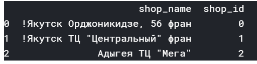
items contain 2 attributes shop_name,item_id ,shop_id
1.4
date date_block_num shop_id item_id item_price item_cnt_day
0 02.01.2013 0 59 22154 999.0 1.0
1 03.01.2013 0 25 2552 899.0 1.0
2 05.01.2013 0 25 2552 899.0 -1.0
train has date,date_block_num ,shop_id,item_id ,item_price ,item_cnt_day
1.5
shop_id item_id
ID
0 5 5037

test has shop_id ,item_id
2.1.data visualing

plt.figure(figsize=(10,4))
plt.xlim(-100, 3000)
sns.boxplot(x=train.item_cnt_day)
plt.figure(figsize=(10,4))
plt.xlim(train.item_price.min(), train.item_price.max()*1.1)
sns.boxplot(x=train.item_price)

the distribution of the item_cnt_day,we can see most data points are below 1000,

the distribution of the item_price,we can see most data points are below 100000,

2.2.data cleaning:

train = train[train.item_price<100000]
train = train[train.item_cnt_day<1001]
print(train[train.item_price<0])

date date_block_num shop_id item_id item_price item_cnt_day
484683 15.05.2013 4 32 2973 -1.0 1.0

median = train[(train.shop_id==32)&(train.item_id==2973)&(train.date_block_num==4)&(train.item_price>0)].item_price.median()
train.loc[train.item_price<0, 'item_price'] = median

so we choose the same shop_id and the same item_id 's media price to represent the price which is below 0
2.3.making the characters spliting and use LabelEncoder to label the characters into numbers

shops['city'] = shops['shop_name'].str.split(' ').map(lambda x: x[0])
shops['city_code'] = LabelEncoder().fit_transform(shops['city'])
shops = shops[['shop_id','city_code']]

before the process:

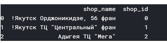
shop_name shop_id
0 !Якутск Орджоникидзе, 56 фран 0
1 !Якутск ТЦ “Центральный” фран 1
2 Адыгея ТЦ “Мега” 2
This is the result：

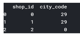
shop_id city_code
0 0 29
1 1 29
2 2 0

2.4.There are 363 item_id which don’t contain in the new test, 5100 test_item_id and 214200 test datasets.

len(list(set(test.item_id) - set(test.item_id).intersection(set(train.item_id)))), len(list(set(test.item_id))), len(test)

(363, 5100, 214200)

2.5.add the total cnt group by date_block_num’,‘shop_id’,'item_id

group = train.groupby(['date_block_num','shop_id','item_id']).agg({'item_cnt_day': ['sum']})
group.columns = ['item_cnt_month']
group.reset_index(inplace=True)

after merge group and train we get 4 attributes and the item_cnt_month has been sumed by group

matrix = pd.merge(matrix, group, on=cols, how='left')
matrix['item_cnt_month'] = (matrix['item_cnt_month']
                                .fillna(0)
                                .clip(0,20) # NB clip target here
                                .astype(np.float16))
print(matrix.head(3))
time.time() - ts

date_block_num shop_id item_id item_cnt_month
0 0 2 19 0.0
1 0 2 27 1.0
2 0 2 28 0.0

2.6
merging the matrix with shops,items,cats get 8 attributes

ts = time.time()
matrix = pd.merge(matrix, shops, on=['shop_id'], how='left')
matrix = pd.merge(matrix, items, on=['item_id'], how='left')
matrix = pd.merge(matrix, cats, on=['item_category_id'], how='left')
matrix['city_code'] = matrix['city_code'].astype(np.int8)
matrix['item_category_id'] = matrix['item_category_id'].astype(np.int8)
matrix['type_code'] = matrix['type_code'].astype(np.int8)
matrix['subtype_code'] = matrix['subtype_code'].astype(np.int8)
time.time() - ts

2.8 using this 8 attributes to train in XGBoost
data=[‘date_block_num’ ,‘shop_id’, ‘item_id’ , ‘item_cnt_month’ , ‘city_code’,‘item_category_id’, ‘type_code’, ‘subtype_code’]

ts = time.time()

model = XGBRegressor(
    max_depth=8,
    n_estimators=10,
    min_child_weight=300, 
    colsample_bytree=0.8, 
    subsample=0.8, 
    eta=0.3,    
    seed=42)

model.fit(
    X_train, 
    Y_train, 
    eval_metric="rmse", 
    eval_set=[(X_train, Y_train), (X_valid, Y_valid)], 
    verbose=True, 
    early_stopping_rounds = 5)

time.time() - ts

第一次提交：