


 本文详细介绍了Kaggle上的一个商品未来销量预测项目,通过对数据的预处理、清洗、分析和模型训练,最终实现对未来销量的预测。在数据预处理阶段,涉及训练集和测试集的处理、商店和商品数据的整合,以及异常值过滤。通过销量和营收分析,揭示了销量下降的原因,并探讨了特定商品对营业收入的影响。在模型训练中,采用LightGBM模型,经过特征工程处理,最终得到预测效果,项目得分0.93740,排名2560/7373。
1. 关于项目
1.1 背景介绍
这是Kaggle竞赛上的一个项目。项目数据由俄罗斯最大的软件公司之一的 1C Company 提供。数据集包含了2013年1月1日到2015年10月31日该公司各商店的商品销售记录。
项目目标是预测该公司接下来2015年11月的商品销量。
项目得分使用RMSD(均方根误差,即得分越低代表预测结果的误差越小,预测效果越好。)进行评估。
项目提交的预测值范围需要在[0,20]。
项目链接:https://www.kaggle.com/c/competitive-data-science-predict-future-sales
1.2项目数据集说明
| 数据集 | 说明 |
|---|---|
| sales_train.csv | 训练集 (包含2013年1月至2015年10月间每天各商店各商品的销量) |
| items.csv | 商品的补充数据集 (包含商品名称和所属分类字段) |
| item_categories.csv | 商品类目的补充数据集 (包含商品所属类目的详细信息) |
| shops.csv | 商店信息的补充数据集 (包含商店所在城市和商店规模的信息) |
| shops.csv test.csv | 测试集 (需要预测的接下来的2015年11月份的各商店的商品销量) |
| sample_submission.csv | 项目提交数据的模板 |
2. 目标
分析该公司的经营状况,找出影响商品销量的相关因素,预测未来一个月该公司各商店不同商品的销量。
3. 数据预处理
3.1 项目数据集预处理
import pandas as pd
import numpy as np
import matplotlib.pyplot as plt
import seaborn as sns
sns.set()
3.1.1 训练集和测试集
train = pd.read_csv('sales_train.csv')
test= pd.read_csv('test.csv')
train.head()
| date | date_block_num | shop_id | item_id | item_price | item_cnt_day | |
|---|---|---|---|---|---|---|
| 0 | 02.01.2013 | 0 | 59 | 22154 | 999.00 | 1.0 |
| 1 | 03.01.2013 | 0 | 25 | 2552 | 899.00 | 1.0 |
| 2 | 05.01.2013 | 0 | 25 | 2552 | 899.00 | -1.0 |
| 3 | 06.01.2013 | 0 | 25 | 2554 | 1709.05 | 1.0 |
| 4 | 15.01.2013 | 0 | 25 | 2555 | 1099.00 | 1.0 |
test.head()
| ID | shop_id | item_id | |
|---|---|---|---|
| 0 | 0 | 5 | 5037 |
| 1 | 1 | 5 | 5320 |
| 2 | 2 | 5 | 5233 |
| 3 | 3 | 5 | 5232 |
| 4 | 4 | 5 | 5268 |
print('训练集的商店数量: %d ,商品数量: %d;\n' % (train['shop_id'].unique().size, train['item_id'].unique().size),
     '测试的商店数量: %d,商品数量: %d。' % (test['shop_id'].unique().size, test['item_id'].unique().size))
训练集的商店数量: 60 ,商品数量: 21807;
 测试的商店数量: 42,商品数量: 5100。
test[~test['shop_id'].isin(train['shop_id'].unique())]
| ID | shop_id | item_id |
|---|
test[~test['item_id'].isin(train['item_id'].unique())]['item_id'].unique()[:10]
array([5320, 5268, 5826, 3538, 3571, 3604, 3407, 3408, 3405, 3984],
      dtype=int64)
测试集里面出现了训练集没有的商品,但是可以根据商店的营销情况和商品类目进行预测。如果直接设置为0的话,反而会使提交的数据成绩减分。这个估计也是要考察模型的泛化能力。
3.1.2 商店数据集
shops = pd.read_csv('shops.csv')
shops.head()
| shop_name | shop_id | |
|---|---|---|
| 0 | !Якутск Орджоникидзе, 56 фран | 0 |
| 1 | !Якутск ТЦ "Центральный" фран | 1 |
| 2 | Адыгея ТЦ "Мега" | 2 |
| 3 | Балашиха ТРК "Октябрь-Киномир" | 3 |
| 4 | Волжский ТЦ "Волга Молл" | 4 |
经过谷歌翻译和百度翻译得知这个是俄罗斯的语言。其中有几个相同商店名称但是不同ID的店铺
- 39号: РостовНаДону ТРК "Мегацентр Горизонт"
- 40号: РостовНаДону ТРК "Мегацентр Горизонт" Островной
上面这两个商店名,差别在最后一个单词,翻译是“岛”,但是在谷歌地图中查找俄罗斯包含“Мегацентр Горизонт”这个名字的购物中心只有РостовНаДону ТРК这个地方上有且只有一个。推测这两个是同一个商店不同叫法。
- 10号: Жуковский ул. Чкалова 39м?
- 11号: Жуковский ул. Чкалова 39м2
这两个推测是书写不一致导致的。
- 0号: !Якутск Орджоникидзе, 56 фран
- 57号: !Якутск Орджоникидзе, 56
这两个也是书写的不一致的问题,类似某某街道56,和某某街道56号的区别。
- 58号:Якутск ТЦ "Центральный"
- 1号: !Якутск ТЦ "Центральный" фран
同上。
- 12 和 56 是线上商店
# 查看测试集是否包含了这几个商店
test[test['shop_id'].isin([39, 40, 10, 11, 0, 57, 58, 1, 12 ,56])]['shop_id'].unique()
array([10, 12, 57, 58, 56, 39], dtype=int64)
测试集中没有包含同一商店的不同ID, 需要对训练集重复商店的不同ID进行修改,修改的ID则以测试集为准。
shop_id_map = {11: 10, 0: 57, 1: 58, 40: 39}
train.loc[train['shop_id'].isin(shop_id_map), 'shop_id'] = train.loc[train['shop_id'].isin(shop_id_map), 'shop_id'].map(shop_id_map)
train.loc[train['shop_id'].isin(shop_id_map), 'shop_id']
Series([], Name: shop_id, dtype: int64)
train.loc[train['shop_id'].isin([39, 40, 10, 11, 0, 57, 58, 1]), 'shop_id'].unique()
array([57, 58, 10, 39], dtype=int64)
对商店名称进行简单分析后,发现商店名称有一个命名规律
大部分商店的名称:
- 开头是一个地区的名称;
- 中间是商店的规模(比如购物中心:ТЦ、大型购物娱乐中心:ТРЦ等);
- 尾部带引号的是商店的名称,比如‘xxx’购物中心,大部分可以在谷歌地图上搜索到。
shops['shop_city'] = shops['shop_name'].map(lambda x:x.split(' ')[0].strip('!'))
shop_types = ['ТЦ', 'ТРК', 'ТРЦ', 'ТК', 'МТРЦ']
shops['shop_type'] = shops['shop_name'].map(lambda x:x.split(' ')[1] if x.split(' ')[1] in shop_types else 'Others')
shops.loc[shops['shop_id'].isin([12, 56]), ['shop_city', 'shop_type']] = 'Online'  # 12和56号是网上商店
shops.head(13)
| shop_name | shop_id | shop_city | shop_type | |
|---|---|---|---|---|
| 0 | !Якутск Орджоникидзе, 56 фран | 0 | Якутск | Others |
| 1 | !Якутск ТЦ "Центральный" фран | 1 | Якутск | ТЦ |
| 2 | Адыгея ТЦ "Мега" | 2 | Адыгея | ТЦ |
| 3 | Балашиха ТРК "Октябрь-Киномир" | 3 | Балашиха | ТРК |
| 4 | Волжский ТЦ "Волга Молл" | 4 | Волжский | ТЦ |
| 5 | Вологда ТРЦ "Мармелад" | 5 | Вологда | ТРЦ |
| 6 | Воронеж (Плехановская, 13) | 6 | Воронеж | Others |
| 7 | Воронеж ТРЦ "Максимир" | 7 | Воронеж | ТРЦ |
| 8 | Воронеж ТРЦ Сити-Парк "Град" | 8 | Воронеж | ТРЦ |
| 9 | Выездная Торговля | 9 | Выездная | Others |
| 10 | Жуковский ул. Чкалова 39м? | 10 | Жуковский | Others |
| 11 | Жуковский ул. Чкалова 39м² | 11 | Жуковский | Others |
| 12 | Интернет-магазин ЧС | 12 | Online | Online |
# 对商店信息进行编码,降低模型训练的内存消耗
shop_city_map = dict([(v,k) for k, v in enumerate(shops['shop_city'].unique())])
shop_type_map = dict([(v,k) for k, v in enumerate(shops['shop_type'].unique())])
shops['shop_city_code'] = shops['shop_city'].map(shop_city_map)
shops['shop_type_code'] = shops['shop_type'].map(shop_type_map)
shops.head(7)
| shop_name | shop_id | shop_city | shop_type | shop_city_code | shop_type_code | |
|---|---|---|---|---|---|---|
| 0 | !Якутск Орджоникидзе, 56 фран | 0 | Якутск | Others | 0 | 0 |
| 1 | !Якутск ТЦ "Центральный" фран | 1 | Якутск | ТЦ | 0 | 1 |
| 2 | Адыгея ТЦ "Мега" | 2 | Адыгея | ТЦ | 1 | 1 |
| 3 | Балашиха ТРК "Октябрь-Киномир" | 3 | Балашиха | ТРК | 2 | 2 |
| 4 | Волжский ТЦ "Волга Молл" | 4 | Волжский | ТЦ | 3 | 1 |
| 5 | Вологда ТРЦ "Мармелад" | 5 | Вологда | ТРЦ | 4 | 3 |
| 6 | Воронеж (Плехановская, 13) | 6 | Воронеж | Others | 5 | 0 |
3.1.3 商品数据集
items = pd.read_csv('items.csv')
items
| item_name | item_id | item_category_id | |
|---|---|---|---|
| 0 | ! ВО ВЛАСТИ НАВАЖДЕНИЯ (ПЛАСТ.) D | 0 | 40 |
| 1 | !ABBYY FineReader 12 Professional Edition Full... | 1 | 76 |
| 2 | ***В ЛУЧАХ СЛАВЫ (UNV) D | 2 | 40 |
| 3 | ***ГОЛУБАЯ ВОЛНА (Univ) D | 3 | 40 |
| 4 | ***КОРОБКА (СТЕКЛО) D | 4 | 40 |
| ... | ... | ... | ... |
| 22165 | Ядерный титбит 2 [PC, Цифровая версия] | 22165 | 31 |
| 22166 | Язык запросов 1С:Предприятия [Цифровая версия] | 22166 | 54 |
| 22167 | Язык запросов 1С:Предприятия 8 (+CD). Хрустале... | 22167 | 49 |
| 22168 | Яйцо для Little Inu | 22168 | 62 |
| 22169 | Яйцо дракона (Игра престолов) | 22169 | 69 |
22170 rows × 3 columns
# 数据集比较大,只分析有没有重复名称不同ID的商品
items['item_name'] = items['item_name'].map(lambda x: ''.join(x.split(' ')))  # 删除空格
duplicated_item_name = items[items['item_name'].duplicated()]
duplicated_item_name
| item_name | item_id | item_category_id | |
|---|---|---|---|
| 2558 | DEEPPURPLEComeHellOrHighWaterDVD | 2558 | 59 |
| 2970 | Divinity:DragonCommander[PC,Цифроваяверсия] | 2970 | 31 |
| 5063 | NIRVANAUnpluggedInNewYorkLP | 5063 | 58 |
| 14539 | МЕНЯЮЩИЕРЕАЛЬНОСТЬ(регион) | 14539 | 40 |
| 19475 | СтругацкиеА.иБ.Улитканасклоне(mp3-CD)(Jewel) | 19475 | 43 |
| 19581 | ТАРЗАН(BD) | 19581 | 37 |
duplicated_item_name_rec = items[items['item_name'].isin(duplicated_item_name['item_name'])]  # 6个商品相同名字不同id的记录
duplicated_item_name_rec
| item_name | item_id | item_category_id | |
|---|---|---|---|
| 2514 | DEEPPURPLEComeHellOrHighWaterDVD | 2514 | 59 |
| 2558 | DEEPPURPLEComeHellOrHighWaterDVD | 2558 | 59 |
| 2968 | Divinity:DragonCommander[PC,Цифроваяверсия] | 2968 | 31 |
| 2970 | Divinity:DragonCommander[PC,Цифроваяверсия] | 2970 | 31 |
| 5061 | NIRVANAUnpluggedInNewYorkLP | 5061 | 58 |
| 5063 | NIRVANAUnpluggedInNewYorkLP | 5063 | 58 |
| 14537 | МЕНЯЮЩИЕРЕАЛЬНОСТЬ(регион) | 14537 | 40 |
| 14539 | МЕНЯЮЩИЕРЕАЛЬНОСТЬ(регион) | 14539 | 40 |
| 19465 | СтругацкиеА.иБ.Улитканасклоне(mp3-CD)(Jewel) | 19465 | 43 |
| 19475 | СтругацкиеА.иБ.Улитканасклоне(mp3-CD)(Jewel) | 19475 | 43 |
| 19579 | ТАРЗАН(BD) | 19579 | 37 |
| 19581 | ТАРЗАН(BD) | 19581 | 37 |
【依旧是查看测试里面包含了哪一些重复项】
test[test['item_id'].isin(duplicated_item_name_rec['item_id'])]['item_id'].unique()
array([19581, 5063], dtype=int64)
【测试集包含了2个同名不同id的商品。且都是较大的ID值。需要把训练集里小的ID值都映射为对应较大的ID值。】
old_id = duplicated_item_name_rec['item_id'].values[::2]
new_id = duplicated_item_name_rec['item_id'].values[1::2]
old_new_map = dict(zip(old_id, new_id))
old_new_map
{2514: 2558, 2968: 2970, 5061: 5063, 14537: 14539, 19465: 19475, 19579: 19581}
train.loc[train['item_id'].isin(old_id), 'item_id'] = train.loc[train['item_id'].isin(old_id), 'item_id'].map(old_new_map)
train[train['item_id'].isin(old_id)]
| date | date_block_num | shop_id | item_id | item_price | item_cnt_day |
|---|
train[train['item_id'].isin(duplicated_item_name_rec['item_id'].values)]['item_id'].unique() # 旧id成功替换成新id
array([ 2558, 14539, 19475, 19581, 5063, 2970], dtype=int64)
3.1.4 商品类目数据集
items.groupby('item_id').size()[items.groupby('item_id').size() > 1] # 检查同一个商品是否分了不同类目
Series([], dtype: int64)
cat = pd.read_csv('item_categories.csv')
cat
| item_category_name | item_category_id | |
|---|---|---|
| 0 | PC - Гарнитуры/Наушники | 0 |
| 1 | Аксессуары - PS2 | 1 |
| 2 | Аксессуары - PS3 | 2 |
| 3 | Аксессуары - PS4 | 3 |
| 4 | Аксессуары - PSP | 4 |
| ... | ... | ... |
| 79 | Служебные | 79 |
| 80 | Служебные - Билеты | 80 |
| 81 | Чистые носители (шпиль) | 81 |
| 82 | Чистые носители (штучные) | 82 |
| 83 | Элементы питания | 83 |
84 rows × 2 columns
cat[cat['item_category_name'].duplicated()]
| item_category_name | item_category_id |
|---|
对类别名称进行简单分析后,发现大部分都是‘大类-小类’的组合形式
Аксессуары :配件
Аксессуары - PS2 :PS2游戏机配件
Игровые консоли :游戏机
【先拆分大类】
cat['item_type'] = cat['item_category_name'].map(lambda x: 'Игры' if x.find('Игры ')>0 else x.split(' -')[0].strip('\"'))
cat.iloc[[32, 33, 34, -3, -2, -1]]  # 有几个比较特殊,需要另外调整一下
| item_category_name | item_category_id | item_type | |
|---|---|---|---|
| 32 | Карты оплаты (Кино, Музыка, Игры) | 32 | Карты оплаты (Кино, Музыка, Игры) |
| 33 | Карты оплаты - Live! | 33 | Карты оплаты |
| 34 | Карты оплаты - Live! (Цифра) | 34 | Карты оплаты |
| 81 | Чистые носители (шпиль) | 81 | Чистые носители (шпиль) |
| 82 | Чистые носители (штучные) | 82 | Чистые носители (штучные) |
| 83 | Элементы питания | 83 | Элементы питания |
cat.iloc[[32,-3, -2], -1] = ['Карты оплаты', 'Чистые носители', 'Чистые носители' ]
cat.iloc[[32,-3, -2]]
| item_category_name | item_category_id | item_type | |
|---|---|---|---|
| 32 | Карты оплаты (Кино, Музыка, Игры) | 32 | Карты оплаты |
| 81 | Чистые носители (шпиль) | 81 | Чистые носители |
| 82 | Чистые носители (штучные) | 82 | Чистые носители |
item_type_map = dict([(v,k) for k, v in enumerate(cat['item_type'].unique())])
cat['item_type_code'] = cat['item_type'].map(item_type_map)
cat.head()
| item_category_name | item_category_id | item_type | item_type_code | |
|---|---|---|---|---|
| 0 | PC - Гарнитуры/Наушники | 0 | PC | 0 |
| 1 | Аксессуары - PS2 | 1 | Аксессуары | 1 |
| 2 | Аксессуары - PS3 | 2 | Аксессуары | 1 |
| 3 | Аксессуары - PS4 | 3 | Аксессуары | 1 |
| 4 | Аксессуары - PSP | 4 | Аксессуары | 1 |
【接着是拆分小类】
cat['sub_type'] = cat['item_category_name'].map(lambda x: x.split('-',1)[-1])
cat
| item_category_name | item_category_id | item_type | item_type_code | sub_type | |
|---|---|---|---|---|---|
| 0 | PC - Гарнитуры/Наушники | 0 | PC | 0 | Гарнитуры/Наушники |
| 1 | Аксессуары - PS2 | 1 | Аксессуары | 1 | PS2 |
| 2 | Аксессуары - PS3 | 2 | Аксессуары | 1 | PS3 |
| 3 | Аксессуары - PS4 | 3 | Аксессуары | 1 | PS4 |
| 4 | Аксессуары - PSP | 4 | Аксессуары | 1 | PSP |
| ... | ... | ... | ... | ... | ... |
| 79 | Служебные | 79 | Служебные | 15 | Служебные |
| 80 | Служебные - Билеты | 80 | Служебные | 15 | Билеты |
| 81 | Чистые носители (шпиль) | 81 | Чистые носители | 16 | Чистые носители (шпиль) |
| 82 | Чистые носители (штучные) | 82 | Чистые носители | 16 | Чистые носители (штучные) |
| 83 | Элементы питания | 83 | Элементы питания | 17 | Элементы питания |
84 rows × 5 columns
cat['sub_type'].unique()
array([' Гарнитуры/Наушники', ' PS2', ' PS3', ' PS4', ' PSP', ' PSVita',
       ' XBOX 360', ' XBOX ONE', 'Билеты (Цифра)', 'Доставка товара',
       ' Прочие', ' Аксессуары для игр', ' Цифра',
       ' Дополнительные издания', ' Коллекционные издания',
       ' Стандартные издания', 'Карты оплаты (Кино, Музыка, Игры)',
       ' Live!', ' Live! (Цифра)', ' PSN', ' Windows (Цифра)', ' Blu-Ray',
       ' Blu-Ray 3D', ' Blu-Ray 4K', ' DVD', ' Коллекционное',
       ' Артбуки, энциклопедии', ' Аудиокниги', ' Аудиокниги (Цифра)',
       ' Аудиокниги 1С', ' Бизнес литература', ' Комиксы, манга',
       ' Компьютерная литература', ' Методические материалы 1С',
       ' Открытки', ' Познавательная литература', ' Путеводители',
       ' Художественная литература', ' CD локального производства',
       ' CD фирменного производства', ' MP3', ' Винил',
       ' Музыкальное видео', ' Подарочные издания', ' Атрибутика',
       ' Гаджеты, роботы, спорт', ' Мягкие игрушки', ' Настольные игры',
       ' Настольные игры (компактные)', ' Открытки, наклейки',
       ' Развитие', ' Сертификаты, услуги', ' Сувениры',
       ' Сувениры (в навеску)', ' Сумки, Альбомы, Коврики д/мыши',
       ' Фигурки', ' 1С:Предприятие 8', ' MAC (Цифра)',
       ' Для дома и офиса', ' Для дома и офиса (Цифра)', ' Обучающие',
       ' Обучающие (Цифра)', 'Служебные', ' Билеты',
       'Чистые носители (шпиль)', 'Чистые носители (штучные)',
       'Элементы питания'], dtype=object)
sub_type_map = dict([(v,k) for k, v in enumerate(cat['sub_type'].unique())])
cat['sub_type_code'] = cat['sub_type'].map(sub_type_map)
cat.head()
| item_category_name | item_category_id | item_type | item_type_code | sub_type | sub_type_code | |
|---|---|---|---|---|---|---|
| 0 | PC - Гарнитуры/Наушники | 0 | PC | 0 | Гарнитуры/Наушники | 0 |
| 1 | Аксессуары - PS2 | 1 | Аксессуары | 1 | PS2 | 1 |
| 2 | Аксессуары - PS3 | 2 | Аксессуары | 1 | PS3 | 2 |
| 3 | Аксессуары - PS4 | 3 | Аксессуары | 1 | PS4 | 3 |
| 4 | Аксессуары - PSP | 4 | Аксессуары | 1 | PSP | 4 |
【合并商品和类目数据集】
items = items.merge(cat[['item_category_id', 'item_type_code', 'sub_type_code']], on='item_category_id', how='left')
items.head()
| item_name | item_id | item_category_id | item_type_code | sub_type_code | |
|---|---|---|---|---|---|
| 0 | !ВОВЛАСТИНАВАЖДЕНИЯ(ПЛАСТ.)D | 0 | 40 | 10 | 24 |
| 1 | !ABBYYFineReader12ProfessionalEditionFull[PC,Ц... | 1 | 76 | 14 | 59 |
| 2 | ***ВЛУЧАХСЛАВЫ(UNV)D | 2 | 40 | 10 | 24 |
| 3 | ***ГОЛУБАЯВОЛНА(Univ)D | 3 | 40 | 10 | 24 |
| 4 | ***КОРОБКА(СТЕКЛО)D | 4 | 40 | 10 | 24 |
import gc
del cat
gc.collect()
2917
3.2 训练集数据清洗
3.2.1 过滤离群值
利用散点图观察商品价格和单日销量的分布情况
sns.jointplot('item_cnt_day', 'item_price', train, kind='scatter')
<seaborn.axisgrid.JointGrid at 0xd6e1d68>

先过滤明显的离群值
train_filtered = train[(train['item_cnt_day'] < 800) & (train['item_price'] < 70000)].copy()
sns.jointplot('item_cnt_day', 'item_price', train_filtered, kind='scatter')
<seaborn.axisgrid.JointGrid at 0xd7bd7b8>

查看价格和销量的异常情况
outer = train[(train['item_cnt_day'] > 400) | (train['item_price'] > 40000)]
outer
| date | date_block_num | shop_id | item_id | item_price | item_cnt_day | |
|---|---|---|---|---|---|---|
| 885138 | 17.09.2013 | 8 | 12 | 11365 | 59200.000000 | 1.0 |
| 1006638 | 24.10.2013 | 9 | 12 | 7238 | 42000.000000 | 1.0 |
| 1163158 | 13.12.2013 | 11 | 12 | 6066 | 307980.000000 | 1.0 |
| 1488135 | 20.03.2014 | 14 | 25 | 13199 | 50999.000000 | 1.0 |
| 1501160 | 15.03.2014 | 14 | 24 | 20949 | 5.000000 | 405.0 |
| 1573252 | 23.04.2014 | 15 | 27 | 8057 | 1200.000000 | 401.0 |
| 1573253 | 22.04.2014 | 15 | 27 | 8057 | 1200.000000 | 502.0 |
| 1708207 | 28.06.2014 | 17 | 25 | 20949 | 5.000000 | 501.0 |
| 2048518 | 02.10.2014 | 21 | 12 | 9242 | 1500.000000 | 512.0 |
| 2067667 | 04.10.2014 | 21 | 55 | 19437 | 899.000000 | 401.0 |
| 2067669 | 09.10.2014 | 21 | 55 | 19437 | 899.000000 | 508.0 |
| 2067677 | 09.10.2014 | 21 | 55 | 19445 | 1249.000000 | 412.0 |
| 2143903 | 20.11.2014 | 22 | 12 | 14173 | 40900.000000 | 1.0 |
| 2257299 | 19.12.2014 | 23 | 12 | 20949 | 4.000000 | 500.0 |
| 2326930 | 15.01.2015 | 24 | 12 | 20949 | 4.000000 | 1000.0 |
| 2327159 | 29.01.2015 | 24 | 12 | 7241 | 49782.000000 | 1.0 |
| 2608040 | 14.04.2015 | 27 | 12 | 3731 | 1904.548077 | 624.0 |
| 2625847 | 19.05.2015 | 28 | 12 | 10209 | 1499.000000 | 480.0 |
| 2626181 | 19.05.2015 | 28 | 12 | 11373 | 155.192950 | 539.0 |
| 2851073 | 29.09.2015 | 32 | 55 | 9249 | 1500.000000 | 533.0 |
| 2851091 | 30.09.2015 | 32 | 55 | 9249 | 1702.825746 | 637.0 |
| 2864235 | 30.09.2015 | 32 | 12 | 9248 | 1692.526158 | 669.0 |
| 2864260 | 29.09.2015 | 32 | 12 | 9248 | 1500.000000 | 504.0 |
| 2885692 | 23.10.2015 | 33 | 42 | 13403 | 42990.000000 | 1.0 |
| 2893100 | 20.10.2015 | 33 | 38 | 13403 | 41990.000000 | 1.0 |
| 2909401 | 14.10.2015 | 33 | 12 | 20949 | 4.000000 | 500.0 |
| 2909818 | 28.10.2015 | 33 | 12 | 11373 | 0.908714 | 2169.0 |
| 2910155 | 20.10.2015 | 33 | 12 | 13403 | 41990.000000 | 1.0 |
| 2910156 | 29.10.2015 | 33 | 12 | 13403 | 42990.000000 | 1.0 |
| 2913267 | 22.10.2015 | 33 | 18 | 13403 | 41990.000000 | 1.0 |
| 2917760 | 20.10.2015 | 33 | 3 | 13403 | 42990.000000 | 1.0 |
| 2927572 | 22.10.2015 | 33 | 28 | 13403 | 40991.000000 | 1.0 |
| 2931380 | 20.10.2015 | 33 | 22 | 13403 | 42990.000000 | 1.0 |
再检查是否需要修改过滤的阈值
outer_set = train_filtered[train_filtered['item_id'].isin(outer['item_id'].unique())].groupby('item_id')

fig, ax = plt.subplots(1,1,figsize=(10, 10))
colors = sns.color_palette() + sns.color_palette('bright')  # 使用调色板。默认颜色只有10来种,会重复使用,不便于观察
i = 1
for name, group in outer_set:
    ax.plot(group['item_cnt_day'], group['item_price'], marker='o', linestyle='', ms=12, label=name, c=colors[i])
    i += 1
ax.legend()

plt.show()

上图可以看出:
1. 青蓝的11365、 橙色的13199 、深红的7241 出现了价格异常高的情况 (大于45000)。(价格在25000 到 45000 是否要考虑)
2. 浅粉的9248、灰色的9249、橘色的3731 出现了销量特别高的情况 (大于600)。(销量高于500的记录也大部分偏离较远,是否需要计入离群值的考量)
train[train['item_id'].isin([13403,7238, 14173])]
| date | date_block_num | shop_id | item_id | item_price | item_cnt_day | |
|---|---|---|---|---|---|---|
| 1006638 | 24.10.2013 | 9 | 12 | 7238 | 42000.0 | 1.0 |
| 2143903 | 20.11.2014 | 22 | 12 | 14173 | 40900.0 | 1.0 |
| 2885692 | 23.10.2015 | 33 | 42 | 13403 | 42990.0 | 1.0 |
| 2885693 | 25.10.2015 | 33 | 42 | 13403 | 28992.0 | 1.0 |
| 2885694 | 29.10.2015 | 33 | 42 | 13403 | 37991.0 | 2.0 |
| 2890617 | 26.10.2015 | 33 | 31 | 13403 | 35991.0 | 1.0 |
| 2893100 | 20.10.2015 | 33 | 38 | 13403 | 41990.0 | 1.0 |
| 2910155 | 20.10.2015 | 33 | 12 | 13403 | 41990.0 | 1.0 |
| 2910156 | 29.10.2015 | 33 | 12 | 13403 | 42990.0 | 1.0 |
| 2913267 | 22.10.2015 | 33 | 18 | 13403 | 41990.0 | 1.0 |
| 2917760 | 20.10.2015 | 33 | 3 | 13403 | 42990.0 | 1.0 |
| 2927572 | 22.10.2015 | 33 | 28 | 13403 | 40991.0 | 1.0 |
| 2931380 | 20.10.2015 | 33 | 22 | 13403 | 42990.0 | 1.0 |
| 2932637 | 26.10.2015 | 33 | 25 | 13403 | 37991.0 | 1.0 |
7238号和14173号只出现过一次,13403号则是新品, 可以考虑过滤掉7238号和214173号
train.loc[train['item_id']==13403].boxplot(['item_cnt_day', 'item_price'])
<matplotlib.axes._subplots.AxesSubplot at 0xf53dc50>

销量高于500的记录中, 蓝色11373和灰色9249的记录看起来明显离群,应该过滤。
剩下的大于400小于600之间的最大值是512。
再查看400到520这中间的商品的销量情况。
m_400 = train[(train['item_cnt_day'] > 400) & (train['item_cnt_day'] < 520)]['item_id'].unique()
n = m_400.size
fig, axes = plt.subplots(1,n,figsize=(n*4, 6))
for i in range(n):
    train[train['item_id'] == m_400[i]].boxplot(['item_cnt_day'], ax=axes[i])
    axes[i].set_title('Item%d' % m_400[i])
plt.show()

销量大于400的记录都偏离其总体水平较远。
总结:
过滤掉7238号和214173号,过滤掉单价高于45000的记录,过滤掉日销量高于400的记录 。
本该查看所有商品销量的离群值。但是数量太多了,耗时且不实际。暂且只过滤与总体差异较为显著的。
况且商品交易本身存在一定的不确定性,去掉全部异常,保留范围内的数据建立的理想化模型来模拟实际情况,结果可能适得其反。保留数据中可接受范围的噪声数据反而更符合实际情况。
filtered = train[(train['item_cnt_day'] < 400) & (train['item_price'] < 45000)].copy()
filtered.head()
| date | date_block_num | shop_id | item_id | item_price | item_cnt_day | |
|---|---|---|---|---|---|---|
| 0 | 02.01.2013 | 0 | 59 | 22154 | 999.00 | 1.0 |
| 1 | 03.01.2013 | 0 | 25 | 2552 | 899.00 | 1.0 |
| 2 | 05.01.2013 | 0 | 25 | 2552 | 899.00 | -1.0 |
| 3 | 06.01.2013 | 0 | 25 | 2554 | 1709.05 | 1.0 |
| 4 | 15.01.2013 | 0 | 25 | 2555 | 1099.00 | 1.0 |
filtered.drop(index=filtered[filtered['item_id'].isin([7238, 14173])].index, inplace=True)
del train, train_filtered
gc.collect()
60
训练集出现销量为-1的情况,估计是出现退货了,属于正常情况。
需要查看有没有小于0的id或者价格。
(filtered[['date_block_num', 'shop_id','item_id', 'item_price']] < 0).any()
date_block_num    False
shop_id           False
item_id           False
item_price         True
dtype: bool
# 商品单价小于0的情况
filtered[filtered['item_price'] <= 0]
| date | date_block_num | shop_id | item_id | item_price | item_cnt_day | |
|---|---|---|---|---|---|---|
| 484683 | 15.05.2013 | 4 | 32 | 2973 | -1.0 | 1.0 |
filtered.groupby(['date_block_num','shop_id', 'item_id'])['item_price'].mean().loc[4, 32, 2973]
1249.0
filtered.loc[filtered['item_price'] <= 0, 'item_price'] = 1249.0  # 用了同一个月同一个商店该商品的均价
filtered[filtered['item_price'] <= 0]  # 检查是否替换成功
| date | date_block_num | shop_id | item_id | item_price | item_cnt_day |
|---|
# 下面也给出替换的函数
def clean_by_mean(df, keys, col):
    """
    用同一月份的均值替换小于等于0的值
    keys 分组键;col 需要替换的字段
    """
    group = df[df[col] <= 0]
    # group = df[df['item_price'] <= 0]
    mean_price = df.groupby(keys)[col].mean()
    # mean_price = df.groupby(['date_block_num', 'shop_id', 'item_id'])['item_price'].mean()
    for i, row in group.iterrows:
        record = group.loc[i]
        df.loc[i,col] = mean_price.loc[record[keys[0]], record[keys[1]], record[keys[2]]]
        # df.loc[i,'item_price'] = mean_price.loc[record['date_block_num'], record['shop_id'], record['item_id']]
    return df
4. 数据规整 和 数据分析(EDA)
# 添加日营业额
filtered['turnover_day'] = filtered['item_price'] * filtered['item_cnt_day']
filtered
| date | date_block_num | shop_id | item_id | item_price | item_cnt_day | turnover_day | |
|---|---|---|---|---|---|---|---|
| 0 | 02.01.2013 | 0 | 59 | 22154 | 999.00 | 1.0 | 999.00 |
| 1 | 03.01.2013 | 0 | 25 | 2552 | 899.00 | 1.0 | 899.00 |
| 2 | 05.01.2013 | 0 | 25 | 2552 | 899.00 | -1.0 | -899.00 |
| 3 | 06.01.2013 | 0 | 25 | 2554 | 1709.05 | 1.0 | 1709.05 |
| 4 | 15.01.2013 | 0 | 25 | 2555 | 1099.00 | 1.0 | 1099.00 |
| ... | ... | ... | ... | ... | ... | ... | ... |
| 2935844 | 10.10.2015 | 33 | 25 | 7409 | 299.00 | 1.0 | 299.00 |
| 2935845 | 09.10.2015 | 33 | 25 | 7460 | 299.00 | 1.0 | 299.00 |
| 2935846 | 14.10.2015 | 33 | 25 | 7459 | 349.00 | 1.0 | 349.00 |
| 2935847 | 22.10.2015 | 33 | 25 | 7440 | 299.00 | 1.0 | 299.00 |
| 2935848 | 03.10.2015 | 33 | 25 | 7460 | 299.00 | 1.0 | 299.00 |
2935824 rows × 7 columns
4.1 销量分析
item_sales_monthly = filtered.pivot_table(columns='item_id',
                                          index='date_block_num',
                                          values='item_cnt_day',
                                          fill_value=0,
                                          aggfunc=sum)
item_sales_monthly.head()
| item_id | 0 | 1 | 2 | 3 | 4 | 5 | 6 | 7 | 8 | 9 | ... | 22160 | 22161 | 22162 | 22163 | 22164 | 22165 | 22166 | 22167 | 22168 | 22169 |
|---|---|---|---|---|---|---|---|---|---|---|---|---|---|---|---|---|---|---|---|---|---|
| date_block_num | |||||||||||||||||||||
| 0 | 0 | 0 | 0 | 0 | 0 | 0 | 0 | 0 | 0 | 0 | ... | 11 | 0 | 0 | 0 | 0 | 0 | 0 | 0 | 2 | 0 |
| 1 | 0 | 0 | 0 | 0 | 0 | 0 | 0 | 0 | 0 | 0 | ... | 7 | 0 | 0 | 0 | 0 | 0 | 0 | 0 | 2 | 0 |
| 2 | 0 | 0 | 0 | 0 | 0 | 0 | 0 | 0 | 0 | 0 | ... | 6 | 0 | 0 | 0 | 0 | 0 | 0 | 0 | 1 | 0 |
| 3 | 0 | 0 | 0 | 0 | 0 | 0 | 0 | 0 | 0 | 0 | ... | 2 | 0 | 0 | 0 | 0 | 0 | 0 | 0 | 0 | 0 |
| 4 | 0 | 0 | 0 | 0 | 0 | 0 | 0 | 0 | 0 | 0 | ... | 6 | 1 | 0 | 0 | 0 | 0 | 0 | 0 | 0 | 0 |
5 rows × 21796 columns
fig, axes = plt.subplots(1,2, figsize=(20, 8))

item_sales_monthly.sum(1).plot(ax=axes[0], title='Total sales of each month', xticks=[i for i in range(0,34,2)])  # 每月总销量
item_sales_monthly.sum(0).plot(ax=axes[1], title='Total sales of each item')  # 每个商品的总销量
plt.subplots_adjust(wspace=0.2)

描述:
总体销量出现下滑趋势,且每月销量大部分都同比下降。
有一款商品的销量异常高。
top_sales = item_sales_monthly.sum().sort_values(ascending=False)
top_sales
item_id
20949    184736
2808      17245
3732      16642
17717     15830
5822      14515
          ...
8515          0
11871        -1
18062        -1
13474        -1
1590        -11
Length: 21796, dtype: int64
test[test['item_id'].isin(top_sales[top_sales<=0].index)]
| ID | shop_id | item_id |
|---|
4.1.1 销量最高的商品
top_sales.iloc[0] / item_sales_monthly.sum().sum() * 100 # 销量占比
5.0801850069973
item_sales_monthly[top_sales.index[0]].plot(kind='bar', figsize=(12,6)) # 每月销量
<matplotlib.axes._subplots.AxesSubplot at 0x1101a240>

item_turnover_monthly = filtered.pivot_table(index= 'date_block_num',
                                               columns= 'item_id',
                                               values='turnover_day',
                                               fill_value=0,
                                               aggfunc=sum)
item_turnover_monthly.head()
| item_id | 0 | 1 | 2 | 3 | 4 | 5 | 6 | 7 | 8 | 9 | ... | 22160 | 22161 | 22162 | 22163 | 22164 | 22165 | 22166 | 22167 | 22168 | 22169 |
|---|---|---|---|---|---|---|---|---|---|---|---|---|---|---|---|---|---|---|---|---|---|
| date_block_num | |||||||||||||||||||||
| 0 | 0 | 0 | 0 | 0 | 0 | 0 | 0 | 0 | 0 | 0 | ... | 1477 | 0 | 0.0 | 0.0 | 0.0 | 0 | 0 | 0.0 | 1598.0 | 0 |
| 1 | 0 | 0 | 0 | 0 | 0 | 0 | 0 | 0 | 0 | 0 | ... | 962 | 0 | 0.0 | 0.0 | 0.0 | 0 | 0 | 0.0 | 1598.0 | 0 |
| 2 | 0 | 0 | 0 | 0 | 0 | 0 | 0 | 0 | 0 | 0 | ... | 894 | 0 | 0.0 | 0.0 | 0.0 | 0 | 0 | 0.0 | 798.5 | 0 |
| 3 | 0 | 0 | 0 | 0 | 0 | 0 | 0 | 0 | 0 | 0 | ... | 298 | 0 | 0.0 | 0.0 | 0.0 | 0 | 0 | 0.0 | 0.0 | 0 |
| 4 | 0 | 0 | 0 | 0 | 0 | 0 | 0 | 0 | 0 | 0 | ... | 894 | 58 | 0.0 | 0.0 | 0.0 | 0 | 0 | 0.0 | 0.0 | 0 |
5 rows × 21796 columns
item_sales_monthly = item_sales_monthly.drop(columns=top_sales[top_sales<=0].index, axis=1)  # 去掉销量为0和负值的商品
item_turnover_monthly = item_turnover_monthly.drop(columns=top_sales[top_sales<=0].index, axis=1)
total_turnover = item_turnover_monthly.sum().sum()
item_turnover_monthly[top_sales.index[0]].sum() / total_turnover * 100
0.02703470087824863
在总销量排名第一的商品,其总销量占到所有总销量的5.080%,但是其总营收却只占到了所有商品总营收的0.027%
items[items['item_id']==20949 ]
| item_name | item_id | item_category_id | item_type_code | sub_type_code | |
|---|---|---|---|---|---|
| 20949 | Фирменныйпакетмайка1СИнтересбелый(34*42)45мкм | 20949 | 71 | 13 | 54 |
翻译过来是一种打包用的包装。该商品的销量依赖于其他需要包装的商品的销售情况。
该产品出现月销量总体下降的情况,说明相应依赖的商品也是总体销量呈下降的趋势。
4.1.2 分析总体销量呈现下降趋势可能存在的原因
使该公司月销量出现总体下降的原因可能存在于两个方面:
一是:商店商品本身热度或生命名周期,等商品内在相关因素,使得商品销量减少。
二是:商品下架或者缺货等外在原因导致商品不再销售,从而影响商品销量。
这两方面的因素不是孤立存在的,对于总体销量来说,这两个影响因素往往是同时存在的。
(item_sales_monthly > 0).sum(1).plot(figsize=(12, 6))
<matplotlib.axes._subplots.AxesSubplot at 0x1e59a860>

2013年每个月在有销量的商品的数量(在售商品数量)都在7500个以上。
2014年每月有销量的商品下降到了约7500-6000个。
2015年则下降到约6500-500个。
小结:在售商品数量呈现总体持续下降的趋势。
item_sales_monthly.sum(1).div((item_sales_monthly > 0).sum(1)).plot(figsize=(12, 6))
# 商品月总销量 / 当月在售商品数量 = 当月在售商品平均销量
<matplotlib.axes._subplots.AxesSubplot at 0x1896d940>

小结:2013年和2014年在售商品月平均销量基本都在13-16个,2015年的在售商品月平均销量则下降到12-14个。
结论:
商品丰富度下降是导致总体销量呈现下降趋势的主要因素之一。
除此之外,2015年在售商品的月均销量相比2013年和2014年下降有所下降,使得2015年总体销量下降幅度高于2013年和2014年。
4.2 营收分析
fig, axes = plt.subplots(1,2, figsize=(20, 8))
item_turnover_monthly.sum(1).plot(ax=axes[0], title='Total turnovers of each month', xticks=[i for i in range(0,34,2)])  # 每月总营收
item_turnover_monthly.sum(0).plot(ax=axes[1], title='Total turnovers of each item')  # 每个商品的总营收
plt.subplots_adjust(wspace=0.2)

描述:
第23个月份的营业收入比第11个月同增长明显,而在销量方面则是同比下跌的。
有一款商品的总营业收入异常的高。
4.2.1 总营收最高的商品
top_turnover = item_turnover_monthly.sum().sort_values(ascending=False)
top_turnover
item_id
6675     2.193915e+08
3732     4.361798e+07
13443    3.433125e+07
3734     3.106516e+07
3733     2.229886e+07
             ...
18098    2.100000e+01
3856     1.700000e+01
7756     1.500000e+01
22010    1.400000e+01
22098    7.000000e+00
Length: 21788, dtype: float64
item_turnover_monthly[top_turnover.index[0]].sum() / total_turnover * 100
6.472732889978659
item_sales_monthly[top_turnover.index[0]].sum() / item_sales_monthly.sum().sum() * 100
0.2829433478063709
在总营业收入排名第一的商品,其销量占总销量的0.28%,其营业收入占公司总营业收入的6.47% 。
item_turnover_monthly[top_turnover.index[0]].plot(kind='bar', figsize=(12, 6))
<matplotlib.axes._subplots.AxesSubplot at 0x18b3b8d0>

item_turnover_monthly[top_turnover.index[0]].div(item_turnover_monthly.sum(1)).plot(figsize=(12, 6),xticks=[i for i in range(0,34,2)])
<matplotlib.axes._subplots.AxesSubplot at 0x18cce588>

items[items['item_id']==top_turnover.index[0]]
| item_name | item_id | item_category_id | item_type_code | sub_type_code | |
|---|---|---|---|---|---|
| 6675 | SonyPlayStation4(500Gb)Black(CUH-1008A/1108A/B01) | 6675 | 12 | 4 | 3 |
这是一款索尼PS4游戏机的一个型号,在13年11月份开始销售,营业收入最的月份为2013年12月,占当月公司总营业收入比例约23%。在15年最后2个月已经没有销量了。
4.3 分析导致14年底销量和营收同比增长趋势不一致的可能原因
turnover_monthly = item_turnover_monthly.sum(1)
sales_monthly = item_sales_monthly.sum(1)
fig, axe1 = plt.subplots(1, 1, figsize=(16, 6))
axe2 = axe1.twinx()
axe1.plot(turnover_monthly.index, turnover_monthly.values, c='r')

axe2.plot(sales_monthly.index, sales_monthly.values, c='b')
axe2.grid(c='c', alpha=0.3)
axe1.legend(['Monthly Turnover'],fontsize=13, bbox_to_anchor=(0.95, 1))
axe2.legend(['Monthly Sales'],fontsize=13, bbox_to_anchor=(0.93, 0.9))
axe1.set_ylabel('Monthly Turnover', c='r')
axe2.set_ylabel('Monthly Sales', c='b')
plt.show()

sales_growth = item_sales_monthly.loc[23].sum() - item_sales_monthly.loc[11].sum()
sales_growth_rate = sales_growth / item_sales_monthly.loc[11].sum() * 100
turnover_growth = item_turnover_monthly.loc[23].sum() - item_turnover_monthly.loc[11].sum()
turnover_growth_rate = turnover_growth / item_turnover_monthly.loc[11].sum() * 100
print(
    ' 销售同比增长量为: %.2f ,同比增长率为: %.2f%%;\n' % (sales_growth, sales_growth_rate),
    '营收同比增长量为: %.2f ,同比增长率为: %.2f%%。' % (turnover_growth, turnover_growth_rate)
     )
 销售同比增长量为: -15086.00 ,同比增长率为: -8.23%;
 营收同比增长量为: 24759419.35 ,同比增长率为: 11.95%。
第23月(2014年12月)销量同比第11月(2013年12月)下降了约15000,但是第23月营业收入同比第11月反而上涨了2500000。
同比增长比率为:销量同比下降8.23%,营业收入同比上涨11.95%。
dec_set = item_turnover_monthly.loc[[11, 23]]
dec_set
| item_id | 0 | 1 | 2 | 3 | 4 | 5 | 6 | 7 | 8 | 9 | ... | 22160 | 22161 | 22162 | 22163 | 22164 | 22165 | 22166 | 22167 | 22168 | 22169 |
|---|---|---|---|---|---|---|---|---|---|---|---|---|---|---|---|---|---|---|---|---|---|
| date_block_num | |||||||||||||||||||||
| 11 | 0 | 0 | 0 | 0 | 0 | 0 | 0 | 0 | 0 | 0 | ... | 0 | 0 | 0.0 | 0.0 | 0.0 | 0 | 4800 | 24613.2 | 0.0 | 0 |
| 23 | 0 | 0 | 0 | 0 | 0 | 28 | 0 | 28 | 0 | 0 | ... | 0 | 0 | 0.0 | 0.0 | 0.0 | 0 | 1650 | 11960.0 | 0.0 | 0 |
2 rows × 21788 columns
观察这两个月份营业收入的分布情况:
plt.figure(figsize=(8, 4))
sns.boxenplot(x=dec_set)
'c' argument looks like a single numeric RGB or RGBA sequence, which should be avoided as value-mapping will have precedence in case its length matches with 'x' & 'y'.  Please use a 2-D array with a single row if you really want to specify the same RGB or RGBA value for all points.


<matplotlib.axes._subplots.AxesSubplot at 0x18b3bf28>

有三款商品的营业收入明显高于其他商品
dec_top = dec_set.loc[:,dec_set.sum() > 5000000]
dec_top  # 年底营收最高的商品
| item_id | 6675 | 13405 | 13443 |
|---|---|---|---|
| date_block_num | |||
| 11 | 4.645973e+07 | 0.000000e+00 | 0.0 |
| 23 | 4.014789e+06 | 7.906979e+06 | 24203004.2 |
在2013年或2014年年底营业收入远超其他商品的商品中,13405号和13443号商品只出现在2014年年底。
可以从新增的这两款商品对营收影响这方面着手分析。
dec_top.iloc[1, 1:].sum() / dec_set.iloc[1].sum() * 100 # 只在第23月出售的商品其营业额占第23个月所有商品营业额的百分比
13.839127677594432
item_sales_monthly.loc[23,dec_top.columns[1:]].sum() / item_sales_monthly.loc[23].sum() * 100
# 13405和13443号商品在第23月销量之和与所有商品总销量的百分比
0.8701078719800304
13405号和13443号商品在2014年12月的营业收入占该月所有商品营业收入的约13.84%,而该月销量只占该月所有总销量的0.87%。
(dec_set.iloc[1].sum() - dec_set.iloc[0].sum()) / dec_set.iloc[0].sum() * 100 # 同比增长率
11.945851204367324
(dec_set.iloc[1].sum() - dec_set.iloc[0].sum()) / dec_set.iloc[1].sum() * 100 # 增长量占总额的百分比
10.67109774578344
item_turnover_monthly[dec_top.columns[1:]].plot(figsize=(12, 6))
<matplotlib.axes._subplots.AxesSubplot at 0x18a29860>

该公司14年12月份营业收入同比增长11.94%,同比增长量占总量10.67%。
而13405号和13443号商品在2014年12月的营业收入占该月所有商品营业收入的约13.84%,超过增长量。
结论:
13405号和13443号商品是该公司14年12月份营业收入同比大幅度增长的主要因素之一。
此外,在前面分析6675号商品中,该商品在2013年12月营收占比约为23%,在2014年的营收占比下降到了约为3%。说明2014年还有其他商品贡献了这约为20%的营业收入。
4.4 帕累托贡献度分析
item_turnover_prop_cumsum = item_turnover_monthly.sum().div(total_turnover).sort_values(ascending=False).cumsum()
pct80 = item_turnover_prop_cumsum.searchsorted(0.8) + 1
pct80_items = item_turnover_prop_cumsum.iloc[:pct80].index
pct80_items
Int64Index([ 6675,  3732, 13443,  3734,  3733, 16787,  3731, 13405, 17717,
             5823,
            ...
             7073, 14333, 15240, 15450,  5581,  3458,  2040,  4837,  1515,
            20658],
           dtype='int64', name='item_id', length=1678)
sales_pct = item_sales_monthly[pct80_items].sum().sum()/ item_sales_monthly.sum().sum()
plt.rcParams['font.sans-serif'] = ['SimHei']
plt.pie([sales_pct, 1 - sales_pct],
        labels=['占总营收80%的商品总销量 ', '占总营收20%的商品总销量 '],
       autopct="%.1f%%",
       textprops={'fontsize':13,'color':"black"},
        startangle=90)
plt.title('帕累托贡献度分析:销量对营收的贡献', fontdict={'fontsize':15,'color':"black"})
plt.show()

小结: 54.2%的商品销量产生了80%的营收效益。45.8%的商品销量只产生了20%的效益。
4.5 店铺对营业收入的贡献
filtered.groupby('shop_id')['item_cnt_day'].sum().sort_values().plot(kind='bar', figsize=(12, 6))
<matplotlib.axes._subplots.AxesSubplot at 0x1e959710>

filtered.groupby('shop_id')['turnover_day'].sum().sort_values().plot(kind='bar', figsize=(12, 6))
<matplotlib.axes._subplots.AxesSubplot at 0x1e6c35c0>

- 对总销量贡献的前三个商店分别是31、25、54号。28号的销量与54号相差不大。
- 对总营业收费贡献的前三个商店分别是31、25、28号。
shops[shops['shop_id'].isin([31, 25, 54, 28])]
| shop_name | shop_id | shop_city | shop_type | shop_city_code | shop_type_code | |
|---|---|---|---|---|---|---|
| 25 | Москва ТРК "Атриум" | 25 | Москва | ТРК | 14 | 2 |
| 28 | Москва ТЦ "МЕГА Теплый Стан" II | 28 | Москва | ТЦ | 14 | 1 |
| 31 | Москва ТЦ "Семеновский" | 31 | Москва | ТЦ | 14 | 1 |
| 54 | Химки ТЦ "Мега" | 54 | Химки | ТЦ | 27 | 1 |
小结:
对总销量和总营业收入贡献前三名的商店都来自同一个城市。
Москва 即:莫斯科,是俄罗斯联邦首都、莫斯科州首府,Химки也是来自莫斯科州,莫斯科州GDP占俄罗斯全国GDP的1/3。
* 商店所在城市的经济规模在很大程度上影响了商店的商品销量。
4.6 产品种类对营业收入的贡献
filtered = filtered.merge(items.iloc[:,1:], on='item_id', how='left')
filtered.head()
| date | date_block_num | shop_id | item_id | item_price | item_cnt_day | turnover_day | item_category_id | item_type_code | sub_type_code | |
|---|---|---|---|---|---|---|---|---|---|---|
| 0 | 02.01.2013 | 0 | 59 | 22154 | 999.00 | 1.0 | 999.00 | 37 | 10 | 21 |
| 1 | 03.01.2013 | 0 | 25 | 2552 | 899.00 | 1.0 | 899.00 | 58 | 12 | 41 |
| 2 | 05.01.2013 | 0 | 25 | 2552 | 899.00 | -1.0 | -899.00 | 58 | 12 | 41 |
| 3 | 06.01.2013 | 0 | 25 | 2554 | 1709.05 | 1.0 | 1709.05 | 58 | 12 | 41 |
| 4 | 15.01.2013 | 0 | 25 | 2555 | 1099.00 | 1.0 | 1099.00 | 56 | 12 | 39 |
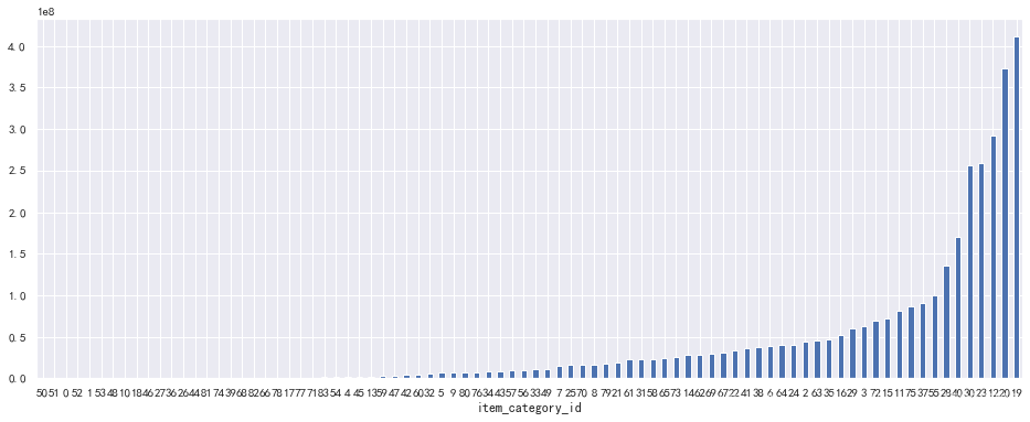
filtered.groupby('item_category_id')['turnover_day'].sum().sort_values().plot(kind='bar',figsize=(16,6), rot=0)
<matplotlib.axes._subplots.AxesSubplot at 0x1e1d31d0>
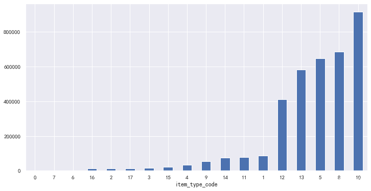
filtered.groupby('item_type_code')['turnover_day'].sum().sort_values().plot(kind='bar',figsize=(12,6), rot=0)
<matplotlib.axes._subplots.AxesSubplot at 0xf7c1438>

filtered.groupby('sub_type_code')['turnover_day'].sum().sort_values().plot(kind='bar',figsize=(12,6), rot=0)
<matplotlib.axes._subplots.AxesSubplot at 0x6c28a20>

小结:
- 商品类目中对总营业收入贡献最大的前三类分别是第19、20、12类。
- 商品大类中第5类商品对总营业收入贡献最大,且与其他类差异明显。
- 商品小类中对总营业收入贡献最大的前三类分别是第3、2、6类。
filtered.groupby('item_category_id')['item_cnt_day'].sum().sort_values().plot(kind='bar',figsize=(16,6), rot=0)
<matplotlib.axes._subplots.AxesSubplot at 0x1e9510f0>

filtered.groupby('item_type_code')['item_cnt_day'].sum().sort_values().plot(kind='bar',figsize=(12,6), rot=0)
<matplotlib.axes._subplots.AxesSubplot at 0x10fc67b8>
filtered.groupby('sub_type_code')['item_cnt_day'].sum().sort_values().plot(kind='bar',figsize=(12,6), rot=0)
<matplotlib.axes._subplots.AxesSubplot at 0x1089d9b0>

小结:
- 商品类目中对总销量贡献最大的前三类分别是第40、30、55类。
- 商品大类中对总销量贡献最大的前三类分别是第10、8、5类,
- 商品小类中对总销量贡献最大的前三类分别是第24、15、38类。
- 在商品大类销量与营业收入综合贡献中,影响最大的是第5和第8类。
- 在商品类目和商品小类中销量和营收前三名中,没有出现重叠的情况。没有综合贡献突出的类。
* 不同种类的商品存在较为明显的销量差异。
4.7 城市和商店类型对营业收入的贡献
filtered = filtered.merge(shops[['shop_id','shop_city_code','shop_type_code']], on='shop_id', how='left')
filtered.head()
| date | date_block_num | shop_id | item_id | item_price | item_cnt_day | turnover_day | item_category_id | item_type_code | sub_type_code | shop_city_code | shop_type_code | |
|---|---|---|---|---|---|---|---|---|---|---|---|---|
| 0 | 02.01.2013 | 0 | 59 | 22154 | 999.00 | 1.0 | 999.00 | 37 | 10 | 21 | 29 | 1 |
| 1 | 03.01.2013 | 0 | 25 | 2552 | 899.00 | 1.0 | 899.00 | 58 | 12 | 41 | 14 | 2 |
| 2 | 05.01.2013 | 0 | 25 | 2552 | 899.00 | -1.0 | -899.00 | 58 | 12 | 41 | 14 | 2 |
| 3 | 06.01.2013 | 0 | 25 | 2554 | 1709.05 | 1.0 | 1709.05 | 58 | 12 | 41 | 14 | 2 |
| 4 | 15.01.2013 | 0 | 25 | 2555 | 1099.00 | 1.0 | 1099.00 | 56 | 12 | 39 | 14 | 2 |
filtered.groupby('shop_city_code')['turnover_day'].sum().plot(kind='bar',figsize=(12,6))
<matplotlib.axes._subplots.AxesSubplot at 0x10895860>

filtered.groupby('shop_type_code')['turnover_day'].sum().plot(kind='bar',figsize=(12,6))
<matplotlib.axes._subplots.AxesSubplot at 0x1af6aac8>

小结: 14区城市的商店对总营业收入贡献最大。1类商店对总营业收入贡献最大。
filtered.groupby('shop_city_code')['item_cnt_day'].sum().plot(kind='bar',figsize=(12,6))
<matplotlib.axes._subplots.AxesSubplot at 0x1b2500b8>

filtered.groupby('shop_type_code')['item_cnt_day'].sum().plot(kind='bar',figsize=(12,6))
<matplotlib.axes._subplots.AxesSubplot at 0x1b27cda0>

小结:
- 在销量方面也是14区城市的商店和1类商店贡献最大。
- 主要影响因素是总营收和总销量排名前三的商店都在14区城市。
* 除了前面分析的商店所在城市会影响商品销量,商店的规模同样在较大程度上影响了商品销量。
题外话:
前面三句红色加粗的话,看起来从常识就可以推断出来了,我在查阅别人的方案时,看到的几乎是直接跳过对这些特征的分析的过程,只给出哪些特征是有用的,容易让人不明所以。
以我个人的理解,通过观测这些特征的值的分布情况,可以直观地了解不同特征对结果影响程度的差异。
而且在后面特征重要性画图时,这些特征的重要性和特征本身对结果影响程度两者之间的一致性,可以作为特征选择可靠性的评判参考。
5. 预测未来销量
5.1 处理关闭的商店和停售的商品
shop_sales_monthly = filtered.pivot_table(index='date_block_num',
                                          columns='shop_id',
                                          values='item_cnt_day',
                                          fill_value=0,
                                          aggfunc=sum)
shop_open_month_cnt = (shop_sales_monthly.iloc[-6:] >  0).sum()  # 有销量的记录
shop_open_month_cnt.head()  # 每个店铺最后半年里有几个月有销量
shop_id
2    6
3    6
4    6
5    6
6    6
dtype: int64
shop_c_n = shop_sales_monthly[shop_open_month_cnt[shop_open_month_cnt < 6].index]
shop_c_n.tail(12)
# 最后半年经营月数少于6个月的店铺
| shop_id | 8 | 9 | 13 | 17 | 20 | 23 | 27 | 29 | 30 | 32 | 33 | 36 | 43 | 51 | 54 |
|---|---|---|---|---|---|---|---|---|---|---|---|---|---|---|---|
| date_block_num | |||||||||||||||
| 22 | 0 | 0 | 0 | 1199 | 0 | 0 | 4675 | 1926 | 2044 | 0 | 814 | 0 | 2659 | 1090 | 6389 |
| 23 | 0 | 0 | 0 | 1832 | 0 | 0 | 7896 | 2402 | 2700 | 0 | 1056 | 0 | 3139 | 1652 | 7677 |
| 24 | 0 | 0 | 0 | 689 | 0 | 0 | 5660 | 1564 | 1842 | 0 | 1006 | 0 | 1340 | 976 | 6043 |
| 25 | 0 | 0 | 0 | 0 | 0 | 0 | 3839 | 1273 | 745 | 0 | 792 | 0 | 0 | 660 | 4221 |
| 26 | 0 | 0 | 0 | 0 | 0 | 0 | 3634 | 1239 | 0 | 0 | 505 | 0 | 0 | 545 | 4625 |
| 27 | 0 | -1 | 0 | 0 | 0 | 0 | 3518 | 1216 | 0 | 0 | -1 | 0 | 0 | 494 | 732 |
| 28 | 0 | 0 | 0 | 0 | 0 | 0 | 3786 | 880 | 0 | 0 | 0 | 0 | 0 | 758 | 0 |
| 29 | 0 | 0 | 0 | 0 | 0 | 0 | 3357 | 0 | 0 | 0 | 0 | 0 | 0 | 659 | 0 |
| 30 | 0 | 0 | 0 | 0 | 0 | 0 | 2478 | 0 | 0 | 0 | 0 | 0 | 0 | 748 | 0 |
| 31 | 0 | 0 | 0 | 0 | 0 | 0 | 0 | 0 | 0 | 0 | 0 | 0 | 0 | 916 | 0 |
| 32 | 0 | 0 | 0 | 0 | 0 | 0 | -1 | 0 | 0 | 0 | 0 | 0 | 0 | 624 | 0 |
| 33 | 0 | 3186 | 0 | 0 | 2611 | 0 | 0 | 0 | 0 | 0 | 0 | 330 | 0 | 0 | 0 |
9, 20, 36 当作是新店,其他的当作已经关闭了
open_shop = shop_sales_monthly[shop_open_month_cnt[shop_open_month_cnt == 6].index]
open_shop.tail(7) # 最后半年都正常经营的商店
| shop_id | 2 | 3 | 4 | 5 | 6 | 7 | 10 | 12 | 14 | 15 | ... | 48 | 49 | 50 | 52 | 53 | 55 | 56 | 57 | 58 | 59 |
|---|---|---|---|---|---|---|---|---|---|---|---|---|---|---|---|---|---|---|---|---|---|
| date_block_num | |||||||||||||||||||||
| 27 | 859 | 740 | 899 | 1054 | 1998 | 1340 | 594 | 2620 | 1055 | 1364 | ... | 1081 | 542 | 895 | 1152 | 1322 | 3422 | 1237 | 2860 | 1710 | 1054 |
| 28 | 843 | 731 | 893 | 1012 | 1748 | 1217 | 466 | 2930 | 933 | 1277 | ... | 1110 | 692 | 1073 | 894 | 1206 | 2117 | 1315 | 2408 | 1378 | 916 |
| 29 | 804 | 672 | 793 | 954 | 1539 | 1235 | 441 | 1830 | 1019 | 1332 | ... | 990 | 789 | 900 | 820 | 1078 | 1909 | 1566 | 2440 | 1554 | 913 |
| 30 | 785 | 535 | 842 | 991 | 1484 | 1327 | 449 | 1554 | 954 | 1316 | ... | 1102 | 856 | 1126 | 828 | 1257 | 1658 | 1491 | 2352 | 1689 | 992 |
| 31 | 942 | 666 | 947 | 1294 | 1575 | 1409 | 442 | 1471 | 1061 | 1360 | ... | 1308 | 966 | 1081 | 932 | 1318 | 1976 | 1604 | 2780 | 1738 | 1214 |
| 32 | 822 | 745 | 732 | 1092 | 1725 | 1287 | 519 | 4042 | 1094 | 1267 | ... | 1101 | 567 | 906 | 1086 | 1229 | 5697 | 1194 | 2266 | 1319 | 914 |
| 33 | 727 | 613 | 831 | 1052 | 1802 | 1212 | 428 | 1512 | 1002 | 1243 | ... | 1111 | 648 | 949 | 847 | 1061 | 1972 | 1263 | 2316 | 1446 | 790 |
7 rows × 41 columns
item_selling_month_cnt = (item_sales_monthly.iloc[-6:] >  0).sum()
item_selling_month_cnt.head()  # 这些商品在最后半年有几个月有销量
item_id
0    0
1    0
2    0
3    0
4    0
dtype: int64
item_zero = item_sales_monthly[item_selling_month_cnt[item_selling_month_cnt == 0].index]
# 这些商品在最后半年都没有销量
item_zero.tail(12)
| item_id | 0 | 1 | 2 | 3 | 4 | 5 | 6 | 7 | 8 | 9 | ... | 22150 | 22151 | 22152 | 22156 | 22157 | 22160 | 22161 | 22165 | 22168 | 22169 |
|---|---|---|---|---|---|---|---|---|---|---|---|---|---|---|---|---|---|---|---|---|---|
| date_block_num | |||||||||||||||||||||
| 22 | 0 | 0 | 1 | 0 | 0 | 0 | 0 | 0 | 0 | 0 | ... | 0 | 0 | 0 | 0 | 0 | 0 | 0 | 0 | 0 | 0 |
| 23 | 0 | 0 | 0 | 0 | 0 | 1 | 0 | 1 | 0 | 0 | ... | 0 | 0 | 0 | 0 | 0 | 0 | 0 | 0 | 0 | 0 |
| 24 | 0 | 0 | 0 | 0 | 0 | 0 | 0 | 0 | 0 | 0 | ... | 0 | 0 | 0 | 0 | 0 | 0 | 0 | 0 | 0 | 0 |
| 25 | 0 | 0 | 0 | 0 | 0 | 0 | 0 | 0 | 0 | 0 | ... | 0 | 0 | 0 | 0 | 0 | 0 | 0 | 0 | 0 | 0 |
| 26 | 0 | 0 | 0 | 0 | 0 | 0 | 0 | 0 | 0 | 0 | ... | 0 | 0 | 0 | 0 | 0 | 0 | 0 | 0 | 0 | 0 |
| 27 | 0 | 0 | 0 | 0 | 0 | 0 | 0 | 0 | 0 | 0 | ... | 0 | 0 | 0 | 0 | 0 | 0 | 0 | 0 | 0 | 0 |
| 28 | 0 | 0 | 0 | 0 | 0 | 0 | 0 | 0 | 0 | 0 | ... | 0 | 0 | 0 | 0 | 0 | 0 | 0 | 0 | 0 | 0 |
| 29 | 0 | 0 | 0 | 0 | 0 | 0 | 0 | 0 | 0 | 0 | ... | 0 | 0 | 0 | 0 | 0 | 0 | 0 | 0 | 0 | 0 |
| 30 | 0 | 0 | 0 | 0 | 0 | 0 | 0 | 0 | 0 | 0 | ... | 0 | 0 | 0 | 0 | 0 | 0 | 0 | 0 | 0 | 0 |
| 31 | 0 | 0 | 0 | 0 | 0 | 0 | 0 | 0 | 0 | 0 | ... | 0 | 0 | 0 | 0 | 0 | 0 | 0 | 0 | 0 | 0 |
| 32 | 0 | 0 | 0 | 0 | 0 | 0 | 0 | 0 | 0 | 0 | ... | 0 | 0 | 0 | 0 | 0 | 0 | 0 | 0 | 0 | 0 |
| 33 | 0 | 0 | 0 | 0 | 0 | 0 | 0 | 0 | 0 | 0 | ... | 0 | 0 | 0 | 0 | 0 | 0 | 0 | 0 | 0 | 0 |
12 rows × 12878 columns
selling_item = item_sales_monthly[item_selling_month_cnt[item_selling_month_cnt > 0].index]
selling_item.tail(12)  # 最后半年有销量的商品
| item_id | 30 | 31 | 32 | 33 | 38 | 39 | 40 | 42 | 45 | 49 | ... | 22153 | 22154 | 22155 | 22158 | 22159 | 22162 | 22163 | 22164 | 22166 | 22167 |
|---|---|---|---|---|---|---|---|---|---|---|---|---|---|---|---|---|---|---|---|---|---|
| date_block_num | |||||||||||||||||||||
| 22 | 13 | 11 | 29 | 20 | 10 | 0 | 1 | 3 | 8 | 3 | ... | 0 | 0 | 0 | 0 | 0 | 0 | 0 | 0 | 16 | 49 |
| 23 | 16 | 18 | 40 | 21 | 11 | 0 | 5 | 2 | 10 | 2 | ... | 1 | 0 | 0 | 0 | 0 | 0 | 0 | 0 | 11 | 40 |
| 24 | 14 | 25 | 42 | 19 | 7 | 0 | 1 | 2 | 11 | 2 | ... | 0 | 0 | 0 | 0 | 0 | 0 | 0 | 0 | 7 | 33 |
| 25 | 14 | 13 | 32 | 26 | 4 | 1 | 1 | 1 | 2 | 4 | ... | 1 | 0 | 0 | 0 | 0 | 311 | 0 | 289 | 8 | 46 |
| 26 | 5 | 12 | 40 | 20 | 1 | 0 | 0 | 2 | 3 | 2 | ... | 0 | 0 | 0 | 0 | 0 | 194 | 0 | 92 | 12 | 40 |
| 27 | 4 | 13 | 20 | 13 | 0 | 0 | 1 | 1 | 5 | 5 | ... | 0 | 0 | 0 | 0 | 0 | 78 | 0 | 27 | 4 | 38 |
| 28 | 5 | 5 | 20 | 12 | 3 | 0 | 0 | 2 | 2 | 2 | ... | 0 | 0 | 0 | 0 | 12 | 35 | 0 | 23 | 8 | 31 |
| 29 | 4 | 10 | 26 | 11 | 2 | 0 | 0 | 1 | 1 | 3 | ... | 0 | 0 | 1 | 0 | 3 | 22 | 0 | 6 | 10 | 33 |
| 30 | 4 | 6 | 21 | 15 | 5 | 0 | 0 | 1 | 3 | 4 | ... | 0 | 8 | 0 | 0 | 0 | 27 | 0 | 12 | 8 | 34 |
| 31 | 6 | 53 | 30 | 14 | 7 | 1 | 0 | 0 | 4 | 4 | ... | 1 | 6 | 0 | 0 | 0 | 14 | 29 | 20 | 11 | 29 |
| 32 | 3 | 9 | 19 | 16 | 2 | 0 | 0 | 1 | 6 | 3 | ... | 0 | 4 | 1 | 0 | 0 | 7 | 20 | 9 | 5 | 21 |
| 33 | 1 | 18 | 22 | 16 | 0 | 0 | 1 | 1 | 1 | 2 | ... | 0 | 5 | 0 | 1 | 0 | 10 | 26 | 15 | 11 | 37 |
12 rows × 8910 columns
5.2 处理训练集
只保留最后6个月正常经营的商店和有销量的商品
cl_set = filtered[filtered['shop_id'].isin(open_shop.columns) & filtered['item_id'].isin(selling_item.columns)]
cl_set
| date | date_block_num | shop_id | item_id | item_price | item_cnt_day | turnover_day | item_category_id | item_type_code | sub_type_code | shop_city_code | shop_type_code | |
|---|---|---|---|---|---|---|---|---|---|---|---|---|
| 0 | 02.01.2013 | 0 | 59 | 22154 | 999.0 | 1.0 | 999.0 | 37 | 10 | 21 | 29 | 1 |
| 1 | 03.01.2013 | 0 | 25 | 2552 | 899.0 | 1.0 | 899.0 | 58 | 12 | 41 | 14 | 2 |
| 2 | 05.01.2013 | 0 | 25 | 2552 | 899.0 | -1.0 | -899.0 | 58 | 12 | 41 | 14 | 2 |
| 10 | 03.01.2013 | 0 | 25 | 2574 | 399.0 | 2.0 | 798.0 | 55 | 12 | 38 | 14 | 2 |
| 11 | 05.01.2013 | 0 | 25 | 2574 | 399.0 | 1.0 | 399.0 | 55 | 12 | 38 | 14 | 2 |
| ... | ... | ... | ... | ... | ... | ... | ... | ... | ... | ... | ... | ... |
| 2935819 | 10.10.2015 | 33 | 25 | 7409 | 299.0 | 1.0 | 299.0 | 55 | 12 | 38 | 14 | 2 |
| 2935820 | 09.10.2015 | 33 | 25 | 7460 | 299.0 | 1.0 | 299.0 | 55 | 12 | 38 | 14 | 2 |
| 2935821 | 14.10.2015 | 33 | 25 | 7459 | 349.0 | 1.0 | 349.0 | 55 | 12 | 38 | 14 | 2 |
| 2935822 | 22.10.2015 | 33 | 25 | 7440 | 299.0 | 1.0 | 299.0 | 57 | 12 | 40 | 14 | 2 |
| 2935823 | 03.10.2015 | 33 | 25 | 7460 | 299.0 | 1.0 | 299.0 | 55 | 12 | 38 | 14 | 2 |
1782392 rows × 12 columns
统计月销量
from itertools import product
import time
ts = time.time()
martix = []
for i in range(34):
    record = cl_set[cl_set['date_block_num'] == i]
    group = product([i],record.shop_id.unique(),record.item_id.unique())
    martix.append(np.array(list(group)))

cols = ['date_block_num', 'shop_id', 'item_id']
martix = pd.DataFrame(np.vstack(martix), columns=cols)

martix
| date_block_num | shop_id | item_id | |
|---|---|---|---|
| 0 | 0 | 59 | 22154 |
| 1 | 0 | 59 | 2552 |
| 2 | 0 | 59 | 2574 |
| 3 | 0 | 59 | 2607 |
| 4 | 0 | 59 | 2515 |
| ... | ... | ... | ... |
| 4940199 | 33 | 21 | 7635 |
| 4940200 | 33 | 21 | 7638 |
| 4940201 | 33 | 21 | 7640 |
| 4940202 | 33 | 21 | 7632 |
| 4940203 | 33 | 21 | 7440 |
4940204 rows × 3 columns
from itertools import product
import time
ts = time.time()
martix = []
for i in range(34):
    record = filtered[filtered['date_block_num'] == i]
    group = product([i],record.shop_id.unique(),record.item_id.unique())
    martix.append(np.array(list(group)))

cols = ['date_block_num', 'shop_id', 'item_id']
martix = pd.DataFrame(np.vstack(martix), columns=cols)

martix
| date_block_num | shop_id | item_id | |
|---|---|---|---|
| 0 | 0 | 59 | 22154 |
| 1 | 0 | 59 | 2552 |
| 2 | 0 | 59 | 2554 |
| 3 | 0 | 59 | 2555 |
| 4 | 0 | 59 | 2564 |
| ... | ... | ... | ... |
| 10840735 | 33 | 21 | 7635 |
| 10840736 | 33 | 21 | 7638 |
| 10840737 | 33 | 21 | 7640 |
| 10840738 | 33 | 21 | 7632 |
| 10840739 | 33 | 21 | 7440 |
10840740 rows × 3 columns
del cl_set
gc.collect()
20
group = filtered.groupby(['date_block_num', 'shop_id', 'item_id']).agg({'item_cnt_day': np.sum})
group.columns = ['item_cnt_month']
group.reset_index(inplace=True)
group
| date_block_num | shop_id | item_id | item_cnt_month | |
|---|---|---|---|---|
| 0 | 0 | 2 | 27 | 1.0 |
| 1 | 0 | 2 | 33 | 1.0 |
| 2 | 0 | 2 | 317 | 1.0 |
| 3 | 0 | 2 | 438 | 1.0 |
| 4 | 0 | 2 | 471 | 2.0 |
| ... | ... | ... | ... | ... |
| 1608242 | 33 | 59 | 22087 | 6.0 |
| 1608243 | 33 | 59 | 22088 | 2.0 |
| 1608244 | 33 | 59 | 22091 | 1.0 |
| 1608245 | 33 | 59 | 22100 | 1.0 |
| 1608246 | 33 | 59 | 22102 | 1.0 |
1608247 rows × 4 columns
martix = pd.merge(martix, group, on=['date_block_num', 'shop_id', 'item_id'], how='left')
martix.head()
| date_block_num | shop_id | item_id | item_cnt_month | |
|---|---|---|---|---|
| 0 | 0 | 59 | 22154 | 1.0 |
| 1 | 0 | 59 | 2552 | NaN |
| 2 | 0 | 59 | 2554 | NaN |
| 3 | 0 | 59 | 2555 | NaN |
| 4 | 0 | 59 | 2564 | NaN |
测试集是第34月的数据,所以给测试集合添加上'date_block_num'字段并设置为34。
待预测的字段‘item_cnt_mun’就设置为0。
test['date_block_num'] = 34
test['item_cnt_month'] = 0
martix = pd.concat([martix.fillna(0), test.drop(columns='ID')], sort=False, ignore_index=True, keys=['date_block_num','shop_id','item_id'])
martix
| date_block_num | shop_id | item_id | item_cnt_month | |
|---|---|---|---|---|
| 0 | 0 | 59 | 22154 | 1.0 |
| 1 | 0 | 59 | 2552 | 0.0 |
| 2 | 0 | 59 | 2554 | 0.0 |
| 3 | 0 | 59 | 2555 | 0.0 |
| 4 | 0 | 59 | 2564 | 0.0 |
| ... | ... | ... | ... | ... |
| 11054935 | 34 | 45 | 18454 | 0.0 |
| 11054936 | 34 | 45 | 16188 | 0.0 |
| 11054937 | 34 | 45 | 15757 | 0.0 |
| 11054938 | 34 | 45 | 19648 | 0.0 |
| 11054939 | 34 | 45 | 969 | 0.0 |
11054940 rows × 4 columns
5.3 特征处理
5.3.1 融合商店数据集和商品数据集的特征
martix = martix.merge(shops[['shop_id', 'shop_type_code', 'shop_city_code']], on='shop_id', how='left')
martix = martix.merge(items.drop(columns='item_name'), on='item_id', how='left')
martix
| date_block_num | shop_id | item_id | item_cnt_month | shop_type_code | shop_city_code | item_category_id | item_type_code | sub_type_code | |
|---|---|---|---|---|---|---|---|---|---|
| 0 | 0 | 59 | 22154 | 1.0 | 1 | 29 | 37 | 10 | 21 |
| 1 | 0 | 59 | 2552 | 0.0 | 1 | 29 | 58 | 12 | 41 |
| 2 | 0 | 59 | 2554 | 0.0 | 1 | 29 | 58 | 12 | 41 |
| 3 | 0 | 59 | 2555 | 0.0 | 1 | 29 | 56 | 12 | 39 |
| 4 | 0 | 59 | 2564 | 0.0 | 1 | 29 | 59 | 12 | 42 |
| ... | ... | ... | ... | ... | ... | ... | ... | ... | ... |
| 11054935 | 34 | 45 | 18454 | 0.0 | 1 | 21 | 55 | 12 | 38 |
| 11054936 | 34 | 45 | 16188 | 0.0 | 1 | 21 | 64 | 13 | 47 |
| 11054937 | 34 | 45 | 15757 | 0.0 | 1 | 21 | 55 | 12 | 38 |
| 11054938 | 34 | 45 | 19648 | 0.0 | 1 | 21 | 40 | 10 | 24 |
| 11054939 | 34 | 45 | 969 | 0.0 | 1 | 21 | 37 | 10 | 21 |
11054940 rows × 9 columns
添加具体的年份和月份
martix['year'] =  martix['date_block_num'].map(lambda x: x // 12 + 2013)
martix['month'] = martix['date_block_num'].map(lambda x: x % 12)
martix.head()
| date_block_num | shop_id | item_id | item_cnt_month | shop_type_code | shop_city_code | item_category_id | item_type_code | sub_type_code | year | month | |
|---|---|---|---|---|---|---|---|---|---|---|---|
| 0 | 0 | 59 | 22154 | 1.0 | 1 | 29 | 37 | 10 | 21 | 2013 | 0 |
| 1 | 0 | 59 | 2552 | 0.0 | 1 | 29 | 58 | 12 | 41 | 2013 | 0 |
| 2 | 0 | 59 | 2554 | 0.0 | 1 | 29 | 58 | 12 | 41 | 2013 | 0 |
| 3 | 0 | 59 | 2555 | 0.0 | 1 | 29 | 56 | 12 | 39 | 2013 | 0 |
| 4 | 0 | 59 | 2564 | 0.0 | 1 | 29 | 59 | 12 | 42 | 2013 | 0 |
5.3.2 添加当月销量特征
当月商店、商品销量均值
# 商品 月销量均值
group = martix.groupby(['date_block_num','item_id']).agg({'item_cnt_month':'mean'})
group.columns = ['item_cnt_month_avg']
group.reset_index(inplace=True)
martix = martix.merge(group, on=['date_block_num', 'item_id'], how='left')
martix.head()
| date_block_num | shop_id | item_id | item_cnt_month | shop_type_code | shop_city_code | item_category_id | item_type_code | sub_type_code | year | month | item_cnt_month_avg | |
|---|---|---|---|---|---|---|---|---|---|---|---|---|
| 0 | 0 | 59 | 22154 | 1.0 | 1 | 29 | 37 | 10 | 21 | 2013 | 0 | 0.400000 |
| 1 | 0 | 59 | 2552 | 0.0 | 1 | 29 | 58 | 12 | 41 | 2013 | 0 | 0.000000 |
| 2 | 0 | 59 | 2554 | 0.0 | 1 | 29 | 58 | 12 | 41 | 2013 | 0 | 0.022222 |
| 3 | 0 | 59 | 2555 | 0.0 | 1 | 29 | 56 | 12 | 39 | 2013 | 0 | 0.044444 |
| 4 | 0 | 59 | 2564 | 0.0 | 1 | 29 | 59 | 12 | 42 | 2013 | 0 | 0.111111 |
# 商店 月销量均值
group = martix.groupby(['date_block_num','shop_id']).agg({'item_cnt_month':'mean'})
group.columns = ['shop_cnt_month_avg']
group.reset_index(inplace=True)
martix = martix.merge(group, on=['date_block_num', 'shop_id'], how='left')
martix.head()
| date_block_num | shop_id | item_id | item_cnt_month | shop_type_code | shop_city_code | item_category_id | item_type_code | sub_type_code | year | month | item_cnt_month_avg | shop_cnt_month_avg | |
|---|---|---|---|---|---|---|---|---|---|---|---|---|---|
| 0 | 0 | 59 | 22154 | 1.0 | 1 | 29 | 37 | 10 | 21 | 2013 | 0 | 0.400000 | 0.248613 |
| 1 | 0 | 59 | 2552 | 0.0 | 1 | 29 | 58 | 12 | 41 | 2013 | 0 | 0.000000 | 0.248613 |
| 2 | 0 | 59 | 2554 | 0.0 | 1 | 29 | 58 | 12 | 41 | 2013 | 0 | 0.022222 | 0.248613 |
| 3 | 0 | 59 | 2555 | 0.0 | 1 | 29 | 56 | 12 | 39 | 2013 | 0 | 0.044444 | 0.248613 |
| 4 | 0 | 59 | 2564 | 0.0 | 1 | 29 | 59 | 12 | 42 | 2013 | 0 | 0.111111 | 0.248613 |
当月种类销量均值
# 类别 月销量均值
group = martix.groupby(['date_block_num','item_category_id']).agg({'item_cnt_month':'mean'})
group.columns = ['cat_cnt_month_avg']
group.reset_index(inplace=True)
martix = martix.merge(group, on=['date_block_num', 'item_category_id'], how='left')
martix.head()
| date_block_num | shop_id | item_id | item_cnt_month | shop_type_code | shop_city_code | item_category_id | item_type_code | sub_type_code | year | month | item_cnt_month_avg | shop_cnt_month_avg | cat_cnt_month_avg | |
|---|---|---|---|---|---|---|---|---|---|---|---|---|---|---|
| 0 | 0 | 59 | 22154 | 1.0 | 1 | 29 | 37 | 10 | 21 | 2013 | 0 | 0.400000 | 0.248613 | 0.199738 |
| 1 | 0 | 59 | 2552 | 0.0 | 1 | 29 | 58 | 12 | 41 | 2013 | 0 | 0.000000 | 0.248613 | 0.043386 |
| 2 | 0 | 59 | 2554 | 0.0 | 1 | 29 | 58 | 12 | 41 | 2013 | 0 | 0.022222 | 0.248613 | 0.043386 |
| 3 | 0 | 59 | 2555 | 0.0 | 1 | 29 | 56 | 12 | 39 | 2013 | 0 | 0.044444 | 0.248613 | 0.049630 |
| 4 | 0 | 59 | 2564 | 0.0 | 1 | 29 | 59 | 12 | 42 | 2013 | 0 | 0.111111 | 0.248613 | 0.093842 |
# 商店-类别 月销量均值
group = martix.groupby(['date_block_num','shop_id','item_category_id']).agg({'item_cnt_month':'mean'})
group.columns = ['shop_cat_cnt_month_avg']
group.reset_index(inplace=True)
martix = martix.merge(group, on=['date_block_num','shop_id','item_category_id'], how='left')
martix.head()
| date_block_num | shop_id | item_id | item_cnt_month | shop_type_code | shop_city_code | item_category_id | item_type_code | sub_type_code | year | month | item_cnt_month_avg | shop_cnt_month_avg | cat_cnt_month_avg | shop_cat_cnt_month_avg | |
|---|---|---|---|---|---|---|---|---|---|---|---|---|---|---|---|
| 0 | 0 | 59 | 22154 | 1.0 | 1 | 29 | 37 | 10 | 21 | 2013 | 0 | 0.400000 | 0.248613 | 0.199738 | 0.088496 |
| 1 | 0 | 59 | 2552 | 0.0 | 1 | 29 | 58 | 12 | 41 | 2013 | 0 | 0.000000 | 0.248613 | 0.043386 | 0.000000 |
| 2 | 0 | 59 | 2554 | 0.0 | 1 | 29 | 58 | 12 | 41 | 2013 | 0 | 0.022222 | 0.248613 | 0.043386 | 0.000000 |
| 3 | 0 | 59 | 2555 | 0.0 | 1 | 29 | 56 | 12 | 39 | 2013 | 0 | 0.044444 | 0.248613 | 0.049630 | 0.008333 |
| 4 | 0 | 59 | 2564 | 0.0 | 1 | 29 | 59 | 12 | 42 | 2013 | 0 | 0.111111 | 0.248613 | 0.093842 | 0.012048 |
# 大类 月销量均值
group = martix.groupby(['date_block_num', 'item_type_code']).agg({'item_cnt_month':'mean'})
group.columns = ['itemtype_cnt_month_avg']
group.reset_index(inplace=True)
martix = martix.merge(group, on=['date_block_num', 'item_type_code'], how='left')
martix.head()
| date_block_num | shop_id | item_id | item_cnt_month | shop_type_code | shop_city_code | item_category_id | item_type_code | sub_type_code | year | month | item_cnt_month_avg | shop_cnt_month_avg | cat_cnt_month_avg | shop_cat_cnt_month_avg | itemtype_cnt_month_avg | |
|---|---|---|---|---|---|---|---|---|---|---|---|---|---|---|---|---|
| 0 | 0 | 59 | 22154 | 1.0 | 1 | 29 | 37 | 10 | 21 | 2013 | 0 | 0.400000 | 0.248613 | 0.199738 | 0.088496 | 0.284744 |
| 1 | 0 | 59 | 2552 | 0.0 | 1 | 29 | 58 | 12 | 41 | 2013 | 0 | 0.000000 | 0.248613 | 0.043386 | 0.000000 | 0.166607 |
| 2 | 0 | 59 | 2554 | 0.0 | 1 | 29 | 58 | 12 | 41 | 2013 | 0 | 0.022222 | 0.248613 | 0.043386 | 0.000000 | 0.166607 |
| 3 | 0 | 59 | 2555 | 0.0 | 1 | 29 | 56 | 12 | 39 | 2013 | 0 | 0.044444 | 0.248613 | 0.049630 | 0.008333 | 0.166607 |
| 4 | 0 | 59 | 2564 | 0.0 | 1 | 29 | 59 | 12 | 42 | 2013 | 0 | 0.111111 | 0.248613 | 0.093842 | 0.012048 | 0.166607 |
# 小类 月销量均值
group = martix.groupby(['date_block_num', 'sub_type_code']).agg({'item_cnt_month':'mean'})
group.columns = ['subtype_cnt_month_avg']
group.reset_index(inplace=True)
martix = martix.merge(group, on=['date_block_num','sub_type_code'], how='left')
martix.head()
| date_block_num | shop_id | item_id | item_cnt_month | shop_type_code | shop_city_code | item_category_id | item_type_code | sub_type_code | year | month | item_cnt_month_avg | shop_cnt_month_avg | cat_cnt_month_avg | shop_cat_cnt_month_avg | itemtype_cnt_month_avg | subtype_cnt_month_avg | |
|---|---|---|---|---|---|---|---|---|---|---|---|---|---|---|---|---|---|
| 0 | 0 | 59 | 22154 | 1.0 | 1 | 29 | 37 | 10 | 21 | 2013 | 0 | 0.400000 | 0.248613 | 0.199738 | 0.088496 | 0.284744 | 0.199738 |
| 1 | 0 | 59 | 2552 | 0.0 | 1 | 29 | 58 | 12 | 41 | 2013 | 0 | 0.000000 | 0.248613 | 0.043386 | 0.000000 | 0.166607 | 0.043386 |
| 2 | 0 | 59 | 2554 | 0.0 | 1 | 29 | 58 | 12 | 41 | 2013 | 0 | 0.022222 | 0.248613 | 0.043386 | 0.000000 | 0.166607 | 0.043386 |
| 3 | 0 | 59 | 2555 | 0.0 | 1 | 29 | 56 | 12 | 39 | 2013 | 0 | 0.044444 | 0.248613 | 0.049630 | 0.008333 | 0.166607 | 0.049630 |
| 4 | 0 | 59 | 2564 | 0.0 | 1 | 29 | 59 | 12 | 42 | 2013 | 0 | 0.111111 | 0.248613 | 0.093842 | 0.012048 | 0.166607 | 0.093842 |
当月商店城市和商店类型的销量均值
# 城市-商品 月销量均值
group = martix.groupby(['date_block_num','shop_city_code','item_id']).agg({'item_cnt_month':'mean'})
group.columns = ['city_item_cnt_month_avg']
group.reset_index(inplace=True)
martix = martix.merge(group, on=['date_block_num','shop_city_code','item_id'], how='left')
martix.head()
| date_block_num | shop_id | item_id | item_cnt_month | shop_type_code | shop_city_code | item_category_id | item_type_code | sub_type_code | year | month | item_cnt_month_avg | shop_cnt_month_avg | cat_cnt_month_avg | shop_cat_cnt_month_avg | itemtype_cnt_month_avg | subtype_cnt_month_avg | city_item_cnt_month_avg | |
|---|---|---|---|---|---|---|---|---|---|---|---|---|---|---|---|---|---|---|
| 0 | 0 | 59 | 22154 | 1.0 | 1 | 29 | 37 | 10 | 21 | 2013 | 0 | 0.400000 | 0.248613 | 0.199738 | 0.088496 | 0.284744 | 0.199738 | 1.0 |
| 1 | 0 | 59 | 2552 | 0.0 | 1 | 29 | 58 | 12 | 41 | 2013 | 0 | 0.000000 | 0.248613 | 0.043386 | 0.000000 | 0.166607 | 0.043386 | 0.0 |
| 2 | 0 | 59 | 2554 | 0.0 | 1 | 29 | 58 | 12 | 41 | 2013 | 0 | 0.022222 | 0.248613 | 0.043386 | 0.000000 | 0.166607 | 0.043386 | 0.0 |
| 3 | 0 | 59 | 2555 | 0.0 | 1 | 29 | 56 | 12 | 39 | 2013 | 0 | 0.044444 | 0.248613 | 0.049630 | 0.008333 | 0.166607 | 0.049630 | 0.0 |
| 4 | 0 | 59 | 2564 | 0.0 | 1 | 29 | 59 | 12 | 42 | 2013 | 0 | 0.111111 | 0.248613 | 0.093842 | 0.012048 | 0.166607 | 0.093842 | 0.0 |
# 商店类型-商品 月销量均值
group = martix.groupby(['date_block_num','shop_type_code','item_id']).agg({'item_cnt_month':'mean'})
group.columns = ['shoptype_item_cnt_month_avg']
group.reset_index(inplace=True)
martix = martix.merge(group, on=['date_block_num','shop_type_code','item_id'], how='left')
martix.head()
| date_block_num | shop_id | item_id | item_cnt_month | shop_type_code | shop_city_code | item_category_id | item_type_code | sub_type_code | year | month | item_cnt_month_avg | shop_cnt_month_avg | cat_cnt_month_avg | shop_cat_cnt_month_avg | itemtype_cnt_month_avg | subtype_cnt_month_avg | city_item_cnt_month_avg | shoptype_item_cnt_month_avg | |
|---|---|---|---|---|---|---|---|---|---|---|---|---|---|---|---|---|---|---|---|
| 0 | 0 | 59 | 22154 | 1.0 | 1 | 29 | 37 | 10 | 21 | 2013 | 0 | 0.400000 | 0.248613 | 0.199738 | 0.088496 | 0.284744 | 0.199738 | 1.0 | 0.28 |
| 1 | 0 | 59 | 2552 | 0.0 | 1 | 29 | 58 | 12 | 41 | 2013 | 0 | 0.000000 | 0.248613 | 0.043386 | 0.000000 | 0.166607 | 0.043386 | 0.0 | 0.00 |
| 2 | 0 | 59 | 2554 | 0.0 | 1 | 29 | 58 | 12 | 41 | 2013 | 0 | 0.022222 | 0.248613 | 0.043386 | 0.000000 | 0.166607 | 0.043386 | 0.0 | 0.00 |
| 3 | 0 | 59 | 2555 | 0.0 | 1 | 29 | 56 | 12 | 39 | 2013 | 0 | 0.044444 | 0.248613 | 0.049630 | 0.008333 | 0.166607 | 0.049630 | 0.0 | 0.04 |
| 4 | 0 | 59 | 2564 | 0.0 | 1 | 29 | 59 | 12 | 42 | 2013 | 0 | 0.111111 | 0.248613 | 0.093842 | 0.012048 | 0.166607 | 0.093842 | 0.0 | 0.12 |
del group
gc.collect()
28
5.3.3 添加销量特征的历史特征
本次项目目标是用历史销量数据预测未来销量。
所以在这里我们转换一下思路,用历史销量数据作为模型的特征,将本月销量结果作为标签建立模型进行回归分析。
def lag_feature(df, lags, col):
    tmp = df[['date_block_num','shop_id','item_id',col]]
    for i in lags:
        shifted = tmp.copy()
        shifted.columns = ['date_block_num','shop_id','item_id', col+'_lag_'+str(i)]
        shifted['date_block_num'] += i
        df = pd.merge(df, shifted, on=['date_block_num','shop_id','item_id'], how='left')
    return df
martix = lag_feature(martix, [1,2,3,6,12], 'item_cnt_month')
martix.head()
| date_block_num | shop_id | item_id | item_cnt_month | shop_type_code | shop_city_code | item_category_id | item_type_code | sub_type_code | year | ... | shop_cat_cnt_month_avg | itemtype_cnt_month_avg | subtype_cnt_month_avg | city_item_cnt_month_avg | shoptype_item_cnt_month_avg | item_cnt_month_lag_1 | item_cnt_month_lag_2 | item_cnt_month_lag_3 | item_cnt_month_lag_6 | item_cnt_month_lag_12 | |
|---|---|---|---|---|---|---|---|---|---|---|---|---|---|---|---|---|---|---|---|---|---|
| 0 | 0 | 59 | 22154 | 1.0 | 1 | 29 | 37 | 10 | 21 | 2013 | ... | 0.088496 | 0.284744 | 0.199738 | 1.0 | 0.28 | NaN | NaN | NaN | NaN | NaN |
| 1 | 0 | 59 | 2552 | 0.0 | 1 | 29 | 58 | 12 | 41 | 2013 | ... | 0.000000 | 0.166607 | 0.043386 | 0.0 | 0.00 | NaN | NaN | NaN | NaN | NaN |
| 2 | 0 | 59 | 2554 | 0.0 | 1 | 29 | 58 | 12 | 41 | 2013 | ... | 0.000000 | 0.166607 | 0.043386 | 0.0 | 0.00 | NaN | NaN | NaN | NaN | NaN |
| 3 | 0 | 59 | 2555 | 0.0 | 1 | 29 | 56 | 12 | 39 | 2013 | ... | 0.008333 | 0.166607 | 0.049630 | 0.0 | 0.04 | NaN | NaN | NaN | NaN | NaN |
| 4 | 0 | 59 | 2564 | 0.0 | 1 | 29 | 59 | 12 | 42 | 2013 | ... | 0.012048 | 0.166607 | 0.093842 | 0.0 | 0.12 | NaN | NaN | NaN | NaN | NaN |
5 rows × 24 columns
martix = lag_feature(martix, [1,2,3,6,12], 'item_cnt_month_avg')
martix = lag_feature(martix, [1,2,3,6,12], 'shop_cnt_month_avg')
martix.head()
| date_block_num | shop_id | item_id | item_cnt_month | shop_type_code | shop_city_code | item_category_id | item_type_code | sub_type_code | year | ... | item_cnt_month_avg_lag_1 | item_cnt_month_avg_lag_2 | item_cnt_month_avg_lag_3 | item_cnt_month_avg_lag_6 | item_cnt_month_avg_lag_12 | shop_cnt_month_avg_lag_1 | shop_cnt_month_avg_lag_2 | shop_cnt_month_avg_lag_3 | shop_cnt_month_avg_lag_6 | shop_cnt_month_avg_lag_12 | |
|---|---|---|---|---|---|---|---|---|---|---|---|---|---|---|---|---|---|---|---|---|---|
| 0 | 0 | 59 | 22154 | 1.0 | 1 | 29 | 37 | 10 | 21 | 2013 | ... | NaN | NaN | NaN | NaN | NaN | NaN | NaN | NaN | NaN | NaN |
| 1 | 0 | 59 | 2552 | 0.0 | 1 | 29 | 58 | 12 | 41 | 2013 | ... | NaN | NaN | NaN | NaN | NaN | NaN | NaN | NaN | NaN | NaN |
| 2 | 0 | 59 | 2554 | 0.0 | 1 | 29 | 58 | 12 | 41 | 2013 | ... | NaN | NaN | NaN | NaN | NaN | NaN | NaN | NaN | NaN | NaN |
| 3 | 0 | 59 | 2555 | 0.0 | 1 | 29 | 56 | 12 | 39 | 2013 | ... | NaN | NaN | NaN | NaN | NaN | NaN | NaN | NaN | NaN | NaN |
| 4 | 0 | 59 | 2564 | 0.0 | 1 | 29 | 59 | 12 | 42 | 2013 | ... | NaN | NaN | NaN | NaN | NaN | NaN | NaN | NaN | NaN | NaN |
5 rows × 34 columns
martix.drop(columns=[ 'item_cnt_month_avg', 'shop_cnt_month_avg'], inplace=True)  # 只保留特征的历史信息
gc.collect()
40
martix = lag_feature(martix, [1,2,3,6,12], 'cat_cnt_month_avg')
martix = lag_feature(martix, [1,2,3,6,12], 'shop_cat_cnt_month_avg')
martix.head()
| date_block_num | shop_id | item_id | item_cnt_month | shop_type_code | shop_city_code | item_category_id | item_type_code | sub_type_code | year | ... | cat_cnt_month_avg_lag_1 | cat_cnt_month_avg_lag_2 | cat_cnt_month_avg_lag_3 | cat_cnt_month_avg_lag_6 | cat_cnt_month_avg_lag_12 | shop_cat_cnt_month_avg_lag_1 | shop_cat_cnt_month_avg_lag_2 | shop_cat_cnt_month_avg_lag_3 | shop_cat_cnt_month_avg_lag_6 | shop_cat_cnt_month_avg_lag_12 | |
|---|---|---|---|---|---|---|---|---|---|---|---|---|---|---|---|---|---|---|---|---|---|
| 0 | 0 | 59 | 22154 | 1.0 | 1 | 29 | 37 | 10 | 21 | 2013 | ... | NaN | NaN | NaN | NaN | NaN | NaN | NaN | NaN | NaN | NaN |
| 1 | 0 | 59 | 2552 | 0.0 | 1 | 29 | 58 | 12 | 41 | 2013 | ... | NaN | NaN | NaN | NaN | NaN | NaN | NaN | NaN | NaN | NaN |
| 2 | 0 | 59 | 2554 | 0.0 | 1 | 29 | 58 | 12 | 41 | 2013 | ... | NaN | NaN | NaN | NaN | NaN | NaN | NaN | NaN | NaN | NaN |
| 3 | 0 | 59 | 2555 | 0.0 | 1 | 29 | 56 | 12 | 39 | 2013 | ... | NaN | NaN | NaN | NaN | NaN | NaN | NaN | NaN | NaN | NaN |
| 4 | 0 | 59 | 2564 | 0.0 | 1 | 29 | 59 | 12 | 42 | 2013 | ... | NaN | NaN | NaN | NaN | NaN | NaN | NaN | NaN | NaN | NaN |
5 rows × 42 columns
martix.drop(columns=['cat_cnt_month_avg', 'shop_cat_cnt_month_avg'], inplace=True)
martix = lag_feature(martix, [1,2,3,6,12], 'itemtype_cnt_month_avg')
martix = lag_feature(martix, [1,2,3,6,12], 'subtype_cnt_month_avg')
martix.head()
| date_block_num | shop_id | item_id | item_cnt_month | shop_type_code | shop_city_code | item_category_id | item_type_code | sub_type_code | year | ... | itemtype_cnt_month_avg_lag_1 | itemtype_cnt_month_avg_lag_2 | itemtype_cnt_month_avg_lag_3 | itemtype_cnt_month_avg_lag_6 | itemtype_cnt_month_avg_lag_12 | subtype_cnt_month_avg_lag_1 | subtype_cnt_month_avg_lag_2 | subtype_cnt_month_avg_lag_3 | subtype_cnt_month_avg_lag_6 | subtype_cnt_month_avg_lag_12 | |
|---|---|---|---|---|---|---|---|---|---|---|---|---|---|---|---|---|---|---|---|---|---|
| 0 | 0 | 59 | 22154 | 1.0 | 1 | 29 | 37 | 10 | 21 | 2013 | ... | NaN | NaN | NaN | NaN | NaN | NaN | NaN | NaN | NaN | NaN |
| 1 | 0 | 59 | 2552 | 0.0 | 1 | 29 | 58 | 12 | 41 | 2013 | ... | NaN | NaN | NaN | NaN | NaN | NaN | NaN | NaN | NaN | NaN |
| 2 | 0 | 59 | 2554 | 0.0 | 1 | 29 | 58 | 12 | 41 | 2013 | ... | NaN | NaN | NaN | NaN | NaN | NaN | NaN | NaN | NaN | NaN |
| 3 | 0 | 59 | 2555 | 0.0 | 1 | 29 | 56 | 12 | 39 | 2013 | ... | NaN | NaN | NaN | NaN | NaN | NaN | NaN | NaN | NaN | NaN |
| 4 | 0 | 59 | 2564 | 0.0 | 1 | 29 | 59 | 12 | 42 | 2013 | ... | NaN | NaN | NaN | NaN | NaN | NaN | NaN | NaN | NaN | NaN |
5 rows × 50 columns
martix.drop(columns=['itemtype_cnt_month_avg', 'subtype_cnt_month_avg'], inplace=True)
martix = lag_feature(martix, [1,2,3,6,12], 'city_item_cnt_month_avg')
martix = lag_feature(martix, [1,2,3,6,12], 'shoptype_item_cnt_month_avg')
martix.head()
| date_block_num | shop_id | item_id | item_cnt_month | shop_type_code | shop_city_code | item_category_id | item_type_code | sub_type_code | year | ... | city_item_cnt_month_avg_lag_1 | city_item_cnt_month_avg_lag_2 | city_item_cnt_month_avg_lag_3 | city_item_cnt_month_avg_lag_6 | city_item_cnt_month_avg_lag_12 | shoptype_item_cnt_month_avg_lag_1 | shoptype_item_cnt_month_avg_lag_2 | shoptype_item_cnt_month_avg_lag_3 | shoptype_item_cnt_month_avg_lag_6 | shoptype_item_cnt_month_avg_lag_12 | |
|---|---|---|---|---|---|---|---|---|---|---|---|---|---|---|---|---|---|---|---|---|---|
| 0 | 0 | 59 | 22154 | 1.0 | 1 | 29 | 37 | 10 | 21 | 2013 | ... | NaN | NaN | NaN | NaN | NaN | NaN | NaN | NaN | NaN | NaN |
| 1 | 0 | 59 | 2552 | 0.0 | 1 | 29 | 58 | 12 | 41 | 2013 | ... | NaN | NaN | NaN | NaN | NaN | NaN | NaN | NaN | NaN | NaN |
| 2 | 0 | 59 | 2554 | 0.0 | 1 | 29 | 58 | 12 | 41 | 2013 | ... | NaN | NaN | NaN | NaN | NaN | NaN | NaN | NaN | NaN | NaN |
| 3 | 0 | 59 | 2555 | 0.0 | 1 | 29 | 56 | 12 | 39 | 2013 | ... | NaN | NaN | NaN | NaN | NaN | NaN | NaN | NaN | NaN | NaN |
| 4 | 0 | 59 | 2564 | 0.0 | 1 | 29 | 59 | 12 | 42 | 2013 | ... | NaN | NaN | NaN | NaN | NaN | NaN | NaN | NaN | NaN | NaN |
5 rows × 58 columns
martix.drop(columns=[ 'city_item_cnt_month_avg','shoptype_item_cnt_month_avg'], inplace=True)
martix
| date_block_num | shop_id | item_id | item_cnt_month | shop_type_code | shop_city_code | item_category_id | item_type_code | sub_type_code | year | ... | city_item_cnt_month_avg_lag_1 | city_item_cnt_month_avg_lag_2 | city_item_cnt_month_avg_lag_3 | city_item_cnt_month_avg_lag_6 | city_item_cnt_month_avg_lag_12 | shoptype_item_cnt_month_avg_lag_1 | shoptype_item_cnt_month_avg_lag_2 | shoptype_item_cnt_month_avg_lag_3 | shoptype_item_cnt_month_avg_lag_6 | shoptype_item_cnt_month_avg_lag_12 | |
|---|---|---|---|---|---|---|---|---|---|---|---|---|---|---|---|---|---|---|---|---|---|
| 0 | 0 | 59 | 22154 | 1.0 | 1 | 29 | 37 | 10 | 21 | 2013 | ... | NaN | NaN | NaN | NaN | NaN | NaN | NaN | NaN | NaN | NaN |
| 1 | 0 | 59 | 2552 | 0.0 | 1 | 29 | 58 | 12 | 41 | 2013 | ... | NaN | NaN | NaN | NaN | NaN | NaN | NaN | NaN | NaN | NaN |
| 2 | 0 | 59 | 2554 | 0.0 | 1 | 29 | 58 | 12 | 41 | 2013 | ... | NaN | NaN | NaN | NaN | NaN | NaN | NaN | NaN | NaN | NaN |
| 3 | 0 | 59 | 2555 | 0.0 | 1 | 29 | 56 | 12 | 39 | 2013 | ... | NaN | NaN | NaN | NaN | NaN | NaN | NaN | NaN | NaN | NaN |
| 4 | 0 | 59 | 2564 | 0.0 | 1 | 29 | 59 | 12 | 42 | 2013 | ... | NaN | NaN | NaN | NaN | NaN | NaN | NaN | NaN | NaN | NaN |
| ... | ... | ... | ... | ... | ... | ... | ... | ... | ... | ... | ... | ... | ... | ... | ... | ... | ... | ... | ... | ... | ... |
| 11054935 | 34 | 45 | 18454 | 0.0 | 1 | 21 | 55 | 12 | 38 | 2015 | ... | 0.5 | 0.0 | 0.0 | 0.0 | NaN | 0.111111 | 0.00 | 0.052632 | 0.666667 | NaN |
| 11054936 | 34 | 45 | 16188 | 0.0 | 1 | 21 | 64 | 13 | 47 | 2015 | ... | 0.0 | 0.0 | NaN | NaN | NaN | 0.000000 | 0.05 | NaN | NaN | NaN |
| 11054937 | 34 | 45 | 15757 | 0.0 | 1 | 21 | 55 | 12 | 38 | 2015 | ... | 0.0 | 0.5 | 0.0 | 0.0 | 0.0 | 0.166667 | 0.10 | 0.105263 | 0.142857 | 0.250000 |
| 11054938 | 34 | 45 | 19648 | 0.0 | 1 | 21 | 40 | 10 | 24 | 2015 | ... | 0.0 | 0.0 | 0.0 | 0.0 | NaN | 0.055556 | 0.05 | 0.263158 | 0.142857 | NaN |
| 11054939 | 34 | 45 | 969 | 0.0 | 1 | 21 | 37 | 10 | 21 | 2015 | ... | 0.5 | 0.0 | 0.0 | 0.0 | 0.0 | 0.111111 | 0.15 | 0.000000 | 0.095238 | 0.041667 |
11054940 rows × 56 columns
martix[martix.columns[:20]].isna().any()
date_block_num              False
shop_id                     False
item_id                     False
item_cnt_month              False
shop_type_code              False
shop_city_code              False
item_category_id            False
item_type_code              False
sub_type_code               False
year                        False
month                       False
item_cnt_month_lag_1         True
item_cnt_month_lag_2         True
item_cnt_month_lag_3         True
item_cnt_month_lag_6         True
item_cnt_month_lag_12        True
item_cnt_month_avg_lag_1     True
item_cnt_month_avg_lag_2     True
item_cnt_month_avg_lag_3     True
item_cnt_month_avg_lag_6     True
dtype: bool
使用之前月份的销量,会导致有很多记录缺失信息。需要将这部分缺失信息的记录去掉。
前面延迟了12个月的销量信息,这里就直接把前12个月的记录删除。
train_set = martix[martix['date_block_num'] > 11].fillna(0)
train_set
| date_block_num | shop_id | item_id | item_cnt_month | shop_type_code | shop_city_code | item_category_id | item_type_code | sub_type_code | year | ... | city_item_cnt_month_avg_lag_1 | city_item_cnt_month_avg_lag_2 | city_item_cnt_month_avg_lag_3 | city_item_cnt_month_avg_lag_6 | city_item_cnt_month_avg_lag_12 | shoptype_item_cnt_month_avg_lag_1 | shoptype_item_cnt_month_avg_lag_2 | shoptype_item_cnt_month_avg_lag_3 | shoptype_item_cnt_month_avg_lag_6 | shoptype_item_cnt_month_avg_lag_12 | |
|---|---|---|---|---|---|---|---|---|---|---|---|---|---|---|---|---|---|---|---|---|---|
| 4487706 | 12 | 54 | 10297 | 4.0 | 1 | 27 | 37 | 10 | 21 | 2014 | ... | 3.0 | 0.0 | 0.0 | 0.0 | 0.0 | 1.080000 | 0.08 | 0.000000 | 0.000000 | 0.000000 |
| 4487707 | 12 | 54 | 10296 | 3.0 | 1 | 27 | 38 | 10 | 22 | 2014 | ... | 0.0 | 0.0 | 0.0 | 0.0 | 0.0 | 0.480000 | 0.00 | 0.000000 | 0.000000 | 0.000000 |
| 4487708 | 12 | 54 | 10298 | 14.0 | 1 | 27 | 40 | 10 | 24 | 2014 | ... | 21.0 | 119.0 | 7.0 | 0.0 | 0.0 | 8.320000 | 33.68 | 3.520000 | 0.000000 | 0.000000 |
| 4487709 | 12 | 54 | 10300 | 3.0 | 1 | 27 | 37 | 10 | 21 | 2014 | ... | 1.0 | 31.0 | 0.0 | 0.0 | 0.0 | 1.040000 | 8.24 | 1.120000 | 0.000000 | 0.000000 |
| 4487710 | 12 | 54 | 10284 | 1.0 | 1 | 27 | 57 | 12 | 40 | 2014 | ... | 0.0 | 0.0 | 0.0 | 1.0 | 0.0 | 0.080000 | 0.04 | 0.160000 | 0.115385 | 0.000000 |
| ... | ... | ... | ... | ... | ... | ... | ... | ... | ... | ... | ... | ... | ... | ... | ... | ... | ... | ... | ... | ... | ... |
| 11054935 | 34 | 45 | 18454 | 0.0 | 1 | 21 | 55 | 12 | 38 | 2015 | ... | 0.5 | 0.0 | 0.0 | 0.0 | 0.0 | 0.111111 | 0.00 | 0.052632 | 0.666667 | 0.000000 |
| 11054936 | 34 | 45 | 16188 | 0.0 | 1 | 21 | 64 | 13 | 47 | 2015 | ... | 0.0 | 0.0 | 0.0 | 0.0 | 0.0 | 0.000000 | 0.05 | 0.000000 | 0.000000 | 0.000000 |
| 11054937 | 34 | 45 | 15757 | 0.0 | 1 | 21 | 55 | 12 | 38 | 2015 | ... | 0.0 | 0.5 | 0.0 | 0.0 | 0.0 | 0.166667 | 0.10 | 0.105263 | 0.142857 | 0.250000 |
| 11054938 | 34 | 45 | 19648 | 0.0 | 1 | 21 | 40 | 10 | 24 | 2015 | ... | 0.0 | 0.0 | 0.0 | 0.0 | 0.0 | 0.055556 | 0.05 | 0.263158 | 0.142857 | 0.000000 |
| 11054939 | 34 | 45 | 969 | 0.0 | 1 | 21 | 37 | 10 | 21 | 2015 | ... | 0.5 | 0.0 | 0.0 | 0.0 | 0.0 | 0.111111 | 0.15 | 0.000000 | 0.095238 | 0.041667 |
6567234 rows × 56 columns
5.3.4 对类别特征进行独热编码、类别编码
lightgbm算法模块的train函数中,有个categorical_feature参数,模型在训练时默认会将Dataframe的category类型字段自动识别为类别特征,就不需要预先对类别特征进行one-hot编码。
很多特征的值的动态范围都比较小,但数据类型默认都是folat64和int64的,非常的占用内存,在训练的时候可能会抛出导致内存不足的异常。这里可以相应地修改成占用内存较低的int32和float32等类型,降低模型训练时的内存压力。
for col in train_set.columns:
    if col.find('code') >= 0:
        train_set[col] = train_set[col].astype(np.int8)
    elif train_set[col].dtype == 'float64':
        train_set[col] = train_set[col].astype(np.float32)
    elif train_set[col].dtype == 'int64':
        train_set[col] = train_set[col].astype(np.int16)

train_set['item_type_code'] = train_set['item_type_code'].astype('category')
train_set['sub_type_code'] = train_set['sub_type_code'].astype('category')
train_set.info()
<class 'pandas.core.frame.DataFrame'>
Int64Index: 6567234 entries, 4487706 to 11054939
Data columns (total 56 columns):
date_block_num                        int16
shop_id                               int16
item_id                               int16
item_cnt_month                        float32
shop_type_code                        int8
shop_city_code                        int8
item_category_id                      int16
item_type_code                        category
sub_type_code                         category
year                                  int16
month                                 int16
item_cnt_month_lag_1                  float32
item_cnt_month_lag_2                  float32
item_cnt_month_lag_3                  float32
item_cnt_month_lag_6                  float32
item_cnt_month_lag_12                 float32
item_cnt_month_avg_lag_1              float32
item_cnt_month_avg_lag_2              float32
item_cnt_month_avg_lag_3              float32
item_cnt_month_avg_lag_6              float32
item_cnt_month_avg_lag_12             float32
shop_cnt_month_avg_lag_1              float32
shop_cnt_month_avg_lag_2              float32
shop_cnt_month_avg_lag_3              float32
shop_cnt_month_avg_lag_6              float32
shop_cnt_month_avg_lag_12             float32
cat_cnt_month_avg_lag_1               float32
cat_cnt_month_avg_lag_2               float32
cat_cnt_month_avg_lag_3               float32
cat_cnt_month_avg_lag_6               float32
cat_cnt_month_avg_lag_12              float32
shop_cat_cnt_month_avg_lag_1          float32
shop_cat_cnt_month_avg_lag_2          float32
shop_cat_cnt_month_avg_lag_3          float32
shop_cat_cnt_month_avg_lag_6          float32
shop_cat_cnt_month_avg_lag_12         float32
itemtype_cnt_month_avg_lag_1          float32
itemtype_cnt_month_avg_lag_2          float32
itemtype_cnt_month_avg_lag_3          float32
itemtype_cnt_month_avg_lag_6          float32
itemtype_cnt_month_avg_lag_12         float32
subtype_cnt_month_avg_lag_1           float32
subtype_cnt_month_avg_lag_2           float32
subtype_cnt_month_avg_lag_3           float32
subtype_cnt_month_avg_lag_6           float32
subtype_cnt_month_avg_lag_12          float32
city_item_cnt_month_avg_lag_1         float32
city_item_cnt_month_avg_lag_2         float32
city_item_cnt_month_avg_lag_3         float32
city_item_cnt_month_avg_lag_6         float32
city_item_cnt_month_avg_lag_12        float32
shoptype_item_cnt_month_avg_lag_1     float32
shoptype_item_cnt_month_avg_lag_2     float32
shoptype_item_cnt_month_avg_lag_3     float32
shoptype_item_cnt_month_avg_lag_6     float32
shoptype_item_cnt_month_avg_lag_12    float32
dtypes: category(2), float32(46), int16(6), int8(2)
memory usage: 1.3 GB
5.4 使用模型训练数据集
这里选择使用lightgbm模型进行训练。
import lightgbm as lgb


X_train = train_set[train_set['date_block_num'] < 33].drop(columns=['item_cnt_month'])  # 训练集的样本特征
Y_train = train_set[train_set['date_block_num'] < 33]['item_cnt_month']  # 训练集的样本标签

X_validate = train_set[train_set['date_block_num'] == 33].drop(columns=['item_cnt_month'])  # 校对集
Y_validate = train_set[train_set['date_block_num'] == 33]['item_cnt_month']

X_test = train_set[train_set['date_block_num'] == 34].drop(columns=['item_cnt_month'])  # 测试集
del train_set
gc.collect()
20
# 把数据加载为模型适合的数据格式
train_data = lgb.Dataset(data=X_train, label=Y_train)
validate_data = lgb.Dataset(data=X_validate, label=Y_validate)
# 设置模型训练参数
import time
ts = time.time()
params = {"objective" : "regression", "metric" : "rmse", 'n_estimators':10000, 'early_stopping_rounds':50,
              "num_leaves" : 200, "learning_rate" : 0.01, "bagging_fraction" : 0.9,
              "feature_fraction" : 0.3, "bagging_seed" : 0}
print('Start....', ts)
lgb_model = lgb.train(params, train_data, valid_sets=[train_data, validate_data], verbose_eval=1000)
print('End...', time.time() - ts)
Start.... 1591718735.6430335


c:\users\honk\appdata\local\programs\python\python37\lib\site-packages\lightgbm\engine.py:148: UserWarning: Found `n_estimators` in params. Will use it instead of argument
  warnings.warn("Found `{}` in params. Will use it instead of argument".format(alias))
c:\users\honk\appdata\local\programs\python\python37\lib\site-packages\lightgbm\engine.py:153: UserWarning: Found `early_stopping_rounds` in params. Will use it instead of argument
  warnings.warn("Found `{}` in params. Will use it instead of argument".format(alias))


Training until validation scores don't improve for 50 rounds
Early stopping, best iteration is:
[152]	training's rmse: 1.95378	valid_1's rmse: 1.57771
End... 330.06891345977783
# 特征重要性画图
lgb.plot_importance(lgb_model, max_num_features=40, figsize=(12, 8))
plt.title("Featurertances")
plt.show()

lgb_model.save_model('model_bestscore02.txt') # 保存模型
<lightgbm.basic.Booster at 0x1e86f1d0>
# 根据项目要求,把数据“裁剪”到[0,20]的区间。
Y_test = lgb_model.predict(X_test).clip(0, 20)
Y_test
array([0.57359759, 0.3126507 , 0.93170284, ..., 0.11140766, 0.10172111,
       0.1178424 ])
X_test['item_cnt_month'] = Y_test
X_test
| date_block_num | shop_id | item_id | shop_type_code | shop_city_code | item_category_id | item_type_code | sub_type_code | year | month | ... | city_item_cnt_month_avg_lag_2 | city_item_cnt_month_avg_lag_3 | city_item_cnt_month_avg_lag_6 | city_item_cnt_month_avg_lag_12 | shoptype_item_cnt_month_avg_lag_1 | shoptype_item_cnt_month_avg_lag_2 | shoptype_item_cnt_month_avg_lag_3 | shoptype_item_cnt_month_avg_lag_6 | shoptype_item_cnt_month_avg_lag_12 | item_cnt_month | |
|---|---|---|---|---|---|---|---|---|---|---|---|---|---|---|---|---|---|---|---|---|---|
| 10840740 | 34 | 5 | 5037 | 3 | 4 | 19 | 5 | 2 | 2015 | 10 | ... | 1.0 | 3.0 | 1.0 | 1.0 | 0.444444 | 2.00 | 4.250000 | 2.500000 | 1.250000 | 0.573598 |
| 10840741 | 34 | 5 | 5320 | 3 | 4 | 55 | 12 | 38 | 2015 | 10 | ... | 0.0 | 0.0 | 0.0 | 0.0 | 0.000000 | 0.00 | 0.000000 | 0.000000 | 0.000000 | 0.312651 |
| 10840742 | 34 | 5 | 5233 | 3 | 4 | 19 | 5 | 2 | 2015 | 10 | ... | 3.0 | 1.0 | 3.0 | 0.0 | 1.222222 | 2.50 | 4.500000 | 2.125000 | 0.000000 | 0.931703 |
| 10840743 | 34 | 5 | 5232 | 3 | 4 | 23 | 5 | 6 | 2015 | 10 | ... | 0.0 | 1.0 | 0.0 | 0.0 | 0.555556 | 1.25 | 2.000000 | 0.000000 | 0.000000 | 0.403808 |
| 10840744 | 34 | 5 | 5268 | 3 | 4 | 20 | 5 | 3 | 2015 | 10 | ... | 0.0 | 0.0 | 0.0 | 0.0 | 0.000000 | 0.00 | 0.000000 | 0.000000 | 0.000000 | 2.331300 |
| ... | ... | ... | ... | ... | ... | ... | ... | ... | ... | ... | ... | ... | ... | ... | ... | ... | ... | ... | ... | ... | ... |
| 11054935 | 34 | 45 | 18454 | 1 | 21 | 55 | 12 | 38 | 2015 | 10 | ... | 0.0 | 0.0 | 0.0 | 0.0 | 0.111111 | 0.00 | 0.052632 | 0.666667 | 0.000000 | 0.172498 |
| 11054936 | 34 | 45 | 16188 | 1 | 21 | 64 | 13 | 47 | 2015 | 10 | ... | 0.0 | 0.0 | 0.0 | 0.0 | 0.000000 | 0.05 | 0.000000 | 0.000000 | 0.000000 | 0.118829 |
| 11054937 | 34 | 45 | 15757 | 1 | 21 | 55 | 12 | 38 | 2015 | 10 | ... | 0.5 | 0.0 | 0.0 | 0.0 | 0.166667 | 0.10 | 0.105263 | 0.142857 | 0.250000 | 0.111408 |
| 11054938 | 34 | 45 | 19648 | 1 | 21 | 40 | 10 | 24 | 2015 | 10 | ... | 0.0 | 0.0 | 0.0 | 0.0 | 0.055556 | 0.05 | 0.263158 | 0.142857 | 0.000000 | 0.101721 |
| 11054939 | 34 | 45 | 969 | 1 | 21 | 37 | 10 | 21 | 2015 | 10 | ... | 0.0 | 0.0 | 0.0 | 0.0 | 0.111111 | 0.15 | 0.000000 | 0.095238 | 0.041667 | 0.117842 |
214200 rows × 56 columns
将预测结果合并到测试集。
result = pd.merge(test[['ID', 'shop_id', 'item_id']],X_test[['shop_id','item_id','item_cnt_month']], on=['shop_id', 'item_id'], how='left')
result
| ID | shop_id | item_id | item_cnt_month | |
|---|---|---|---|---|
| 0 | 0 | 5 | 5037 | 0.573598 |
| 1 | 1 | 5 | 5320 | 0.312651 |
| 2 | 2 | 5 | 5233 | 0.931703 |
| 3 | 3 | 5 | 5232 | 0.403808 |
| 4 | 4 | 5 | 5268 | 2.331300 |
| ... | ... | ... | ... | ... |
| 214195 | 214195 | 45 | 18454 | 0.172498 |
| 214196 | 214196 | 45 | 16188 | 0.118829 |
| 214197 | 214197 | 45 | 15757 | 0.111408 |
| 214198 | 214198 | 45 | 19648 | 0.101721 |
| 214199 | 214199 | 45 | 969 | 0.117842 |
214200 rows × 4 columns
result.isna().any()
ID                False
shop_id           False
item_id           False
item_cnt_month    False
dtype: bool
前面分析关闭的商店中,有3个商在最近半年里只有最后一个月有销量,推断是新开的商店。
还有一些商品是最近半年都没有销量,推断是已经下架的商品,预测值填为0 。
result[result.shop_id.isin(shop_c_n.columns)]['shop_id'].unique()
array([36], dtype=int64)
result.loc[result.item_id.isin(item_zero), 'item_cnt_month'] = 0
result.loc[result.item_id.isin(item_zero), 'item_cnt_month']
298       0.0
493       0.0
817       0.0
953       0.0
1165      0.0
         ...
214165    0.0
214167    0.0
214176    0.0
214179    0.0
214180    0.0
Name: item_cnt_month, Length: 7812, dtype: float64
result[['ID','item_cnt_month']].to_csv('fromfinal01.csv',sep=',',index=False)
5.5 预测效果评估
得分:0.93740

当前排名:2560/7373
6. 项目总结
项目经验:
本次项目花了几个星期的业余时间才完成的,花费了很多精力和时间,但总算是有所收获。
从数据分析方法到特征工程和预测模型的构建,都花了很多时间去研究和梳理。通过这次项目学到了很多,包括问题切入的有效面、分析算法的代码实现,分析流程的设计等,让我从整体上更好的掌握数据分析的思维。
项目不足:
- 数据分析方法分两种:一种是统计分析方法,另一种是挖掘方法。在做预测型分析的时候,特征分析和模型构建往往都需要用到数据挖掘的方法和思维,在这个一方面的理论和数据支撑还不够简明有力,还需要加强学习。
- 在特征处理中,还有一个商品价格的特征没有加入到预测模型里面。主要原因是对价格特征的处理还存在一些不足之处,价格特征比较特殊,和销量不一样,如果某商品当月没有销量的话,销量可以记为0,但是价格则不能记录为0 。我的做法是使用最近半年内上次有销量的价格,但是预测效果并不好,需要重新理解这内在的联系,重新构建价格特征。


 2230
2230

 被折叠的 条评论
为什么被折叠?
被折叠的 条评论
为什么被折叠?
 到【灌水乐园】发言


