


Predict Future Sales
- 数据分析
- 1. 数据基本处理
- 2. 数据探索
- 3 特征融合
- 3.1 统计月销量
- 3.2 相关信息融合
- 3.2 历史信息
- 3.2.1 lag operation产生延迟信息,可以选择延迟的月数。
- 3.2.2 月销量(每个商品-商店)的历史信息
- 3.2.3 月销量(所有商品-商店)均值的历史信息
- 3.2.4 月销量(每件商品)均值和历史特征
- 3.2.5 月销量(每个商店)均值和历史特征
- 3.2.6 月销量(每个商品类别)均值和历史特征
- 3.2.7 月销量(商品类别-商店)均值和历史特征
- 3.2.8 月销量(商品类别_大类)均值和历史特征
- 3.2.9 月销量(商品-商品类别_大类)均值和历史特征
- 3.2.10 月销量(商店_城市)均值和历史特征
- 3.2.11 月销量(商品-商店_城市)均值和历史特征
- 3.2.12 趋势特征,半年来价格的变化
- 3.2.13 每个月天数
- 3.2.14 开始和结束的销量
- 4. 数据建模
预测未来销售该项目来源于kaggle中的一场比赛的赛题,数据是由日常销售数据组成的时间序列数据集,该数据集由俄罗斯最大的软件公司之一 - 1C公司提供。提供了包括商店,商品,价格,日销量等连续34个月内的数据,要求预测第35个月的各商店各商品的销量。评价指标为RMSE,Baseline是1.1677,我的成绩是0.89896,目前排名178/3200。
| 文件名 | 文件说明 |
|---|---|
| sales_train.csv | 训练集(date_block=0 到 33 的每日历史数据,包括各商品在各商店的销量,价格) |
| test.csv | 测试集(date_block=34 的商店和产品信息) |
| items.csv | 商品的详细信息(item_name、item_id、item_category_id) |
| item_categories.csv | 商品类别的详细信息(item_category_name、item_category_id) |
| shops.csv | 商店的详细信息(shop_name、shop_id) |
数据分析
1. 数据基本处理
1.1 读入数据集
- 训练集有六列,分别介绍日期,月份,商店,商品,价格和日销量
- 测试集有三列,分别是ID,商店,和商品。
sales_train = pd.read_csv('input/sales_train.csv.gz')
test = pd.read_csv('input/test.csv.gz')
sales_train.head()
| date | date_block_num | shop_id | item_id | item_price | item_cnt_day | |
|---|---|---|---|---|---|---|
| 0 | 02.01.2013 | 0 | 59 | 22154 | 999.00 | 1.0 |
| 1 | 03.01.2013 | 0 | 25 | 2552 | 899.00 | 1.0 |
| 2 | 05.01.2013 | 0 | 25 | 2552 | 899.00 | -1.0 |
| 3 | 06.01.2013 | 0 | 25 | 2554 | 1709.05 | 1.0 |
| 4 | 15.01.2013 | 0 | 25 | 2555 | 1099.00 | 1.0 |
test.head()
| ID | shop_id | item_id | |
|---|---|---|---|
| 0 | 0 | 5 | 5037 |
| 1 | 1 | 5 | 5320 |
| 2 | 2 | 5 | 5233 |
| 3 | 3 | 5 | 5232 |
| 4 | 4 | 5 | 5268 |
- 训练集,有21807种商品,60个商店。一共2935849 种商品-商店组合。
- 测试集,有5100 种商品,42个商店。刚好就是5100 * 42 = 214200种 商品-商店组合。
print('how many lines in train set:', sales_train.shape)
print('unique items in train set:', sales_train['item_id'].nunique())
print('unique shops in train set:', sales_train['shop_id'].nunique())
print('how many lines in test set:', test.shape)
print('unique items in test set:', test['item_id'].nunique())
print('unique shops in test set:', test['shop_id'].nunique())
how many lines in train set: (2935849, 6)
unique items in train set: 21807
unique shops in train set: 60
how many lines in test set: (214200, 3)
unique items in test set: 5100
unique shops in test set: 42
查看数据的基本信息以及是否有数据缺失NAN
数据形状为(2935849, 6),sales_train中没有missing values,没有nan,
print('----------head---------')
print(sales_train.head(5))
print('------information------')
print(sales_train.info())
print('-----missing value-----')
print(sales_train.isnull().sum())
print('--------nan value------')
print(sales_train.isna().sum())
----------head---------
         date  date_block_num  shop_id  item_id  item_price  item_cnt_day
0  02.01.2013               0       59    22154      999.00           1.0
1  03.01.2013               0       25     2552      899.00           1.0
2  05.01.2013               0       25     2552      899.00          -1.0
3  06.01.2013               0       25     2554     1709.05           1.0
4  15.01.2013               0       25     2555     1099.00           1.0
------information------
<class 'pandas.core.frame.DataFrame'>
RangeIndex: 2935849 entries, 0 to 2935848
Data columns (total 6 columns):
date              object
date_block_num    int64
shop_id           int64
item_id           int64
item_price        float64
item_cnt_day      float64
dtypes: float64(2), int64(3), object(1)
memory usage: 134.4+ MB
None
-----missing value-----
date              0
date_block_num    0
shop_id           0
item_id           0
item_price        0
item_cnt_day      0
dtype: int64
--------nan value------
date              0
date_block_num    0
shop_id           0
item_id           0
item_price        0
item_cnt_day      0
dtype: int64
1.2 基线模型预测
首先尝试复现基线模型。本次比赛中,基线模型就是用第34个月的销售当作第35个月的销售,即将2015年10月的结果当作2015年11月的预测。评估结果应该是1.16777.
- 训练集中的数据是 商品-商店-每天的销售。而要求预测的是商品-商店-每月的销售,因此需要合理使用groupby()和agg()函数。
- 训练集没有出现过的 商品-商店组合,一律填零,最终的结果需要限幅在 [0,20]区间。
sales_train_subset = sales_train[sales_train['date_block_num'] == 33]
sales_train_subset.head()

grouped = sales_train_subset[['shop_id','item_id','item_cnt_day']].groupby(['shop_id','item_id']).agg({'item_cnt_day':'sum'}).reset_index()
grouped = grouped.rename(columns={'item_cnt_day' : 'item_cnt_month'})
grouped.head()
| shop_id | item_id | item_cnt_month | |
|---|---|---|---|
| 0 | 2 | 31 | 1.0 |
| 1 | 2 | 486 | 3.0 |
| 2 | 2 | 787 | 1.0 |
| 3 | 2 | 794 | 1.0 |
| 4 | 2 | 968 | 1.0 |
test = pd.read_csv('../readonly/final_project_data/test.csv.gz')
test = pd.merge(test,grouped, on = ['shop_id','item_id'], how = 'left')
print(test.head())
test['item_cnt_month'] = test['item_cnt_month'].fillna(0).clip(0,20)
print(test.head())
test = test[['ID','item_cnt_month']]
submission = test.set_index('ID')
submission.to_csv('submission_baseline.csv')
   ID  shop_id  item_id  item_cnt_month
0   0        5     5037             NaN
1   1        5     5320             NaN
2   2        5     5233             1.0
3   3        5     5232             NaN
4   4        5     5268             NaN
   ID  shop_id  item_id  item_cnt_month
0   0        5     5037             0.0
1   1        5     5320             0.0
2   2        5     5233             1.0
3   3        5     5232             0.0
4   4        5     5268             0.0
1.3 节省存储空间
因为后续会做大量的特征提取,对存储空间的消耗较大,而且较大的特征集对于模型训练来说也是个负担。在训练集中可以发现,很多数据的动态范围很小,比如date_block_num,shop_id,item_id,用int16存储就足够了。而Item_price, item_cnt_day 用float32 存储也是足够的。这样就可以在不损失信息的前提下,减少一般的存储空间消耗。结果来看从134.4+ MB,减少到了 61.6+ MB。
def downcast_dtypes(df):
    cols_float64 = [c for c in df if df[c].dtype == 'float64']
    cols_int64_32 = [c for c in df if df[c].dtype in ['int64', 'int32']]
    df[cols_float64] = df[cols_float64].astype(np.float32)
    df[cols_int64_32] = df[cols_int64_32].astype(np.int16)
    return df
sales_train = downcast_dtypes(sales_train)
test = downcast_dtypes(test)
sales_train.info()
<class 'pandas.core.frame.DataFrame'>
RangeIndex: 2935849 entries, 0 to 2935848
Data columns (total 6 columns):
date              object
date_block_num    int16
shop_id           int16
item_id           int16
item_price        float32
item_cnt_day      float32
dtypes: float32(2), int16(3), object(1)
memory usage: 61.6+ MB
2. 数据探索
2.1 训练集分析 sales_train
2.1.1 每件商品的销量
我们使用pivot_table来查看每件商品每个月的销量。pivot_table()和groupby()的用途类似,但更加灵活,可以对columns做更多处理。
sales_by_item_id = sales_train.pivot_table(index=['item_id'],values=['item_cnt_day'],
                                        columns='date_block_num', aggfunc=np.sum, fill_value=0).reset_index()
sales_by_item_id.columns = sales_by_item_id.columns.droplevel().map(str)
sales_by_item_id = sales_by_item_id.reset_index(drop=True).rename_axis(None, axis=1)
sales_by_item_id.columns.values[0] = 'item_id'
sales_by_item_id.tail()
| item_id | 0 | 1 | 2 | 3 | 4 | 5 | 6 | 7 | 8 | 9 | 10 | 11 | 12 | 13 | 14 | 15 | 16 | 17 | 18 | 19 | 20 | 21 | 22 | 23 | 24 | 25 | 26 | 27 | 28 | 29 | 30 | 31 | 32 | 33 | |
|---|---|---|---|---|---|---|---|---|---|---|---|---|---|---|---|---|---|---|---|---|---|---|---|---|---|---|---|---|---|---|---|---|---|---|---|
| 21802 | 22165 | 0 | 0 | 0 | 0 | 0 | 0 | 0 | 1 | 0 | 0 | 0 | 0 | 0 | 0 | 0 | 0 | 1 | 0 | 0 | 0 | 0 | 0 | 0 | 0 | 0 | 0 | 0 | 0 | 0 | 0 | 0 | 0 | 0 | 0 |
| 21803 | 22166 | 0 | 0 | 0 | 0 | 0 | 0 | 0 | 0 | 0 | 23 | 24 | 32 | 25 | 24 | 21 | 13 | 10 | 15 | 12 | 13 | 13 | 12 | 16 | 11 | 7 | 8 | 12 | 4 | 8 | 10 | 8 | 11 | 5 | 11 |
| 21804 | 22167 | 0 | 0 | 0 | 0 | 0 | 0 | 0 | 0 | 56 | 146 | 96 | 83 | 66 | 57 | 47 | 59 | 41 | 56 | 47 | 47 | 39 | 49 | 49 | 40 | 33 | 46 | 40 | 38 | 31 | 33 | 34 | 29 | 21 | 37 |
| 21805 | 22168 | 2 | 2 | 1 | 0 | 0 | 0 | 0 | 0 | 1 | 0 | 0 | 0 | 0 | 0 | 0 | 0 | 0 | 0 | 0 | 0 | 0 | 0 | 0 | 0 | 0 | 0 | 0 | 0 | 0 | 0 | 0 | 0 | 0 | 0 |
| 21806 | 22169 | 0 | 0 | 0 | 0 | 0 | 0 | 0 | 0 | 0 | 0 | 0 | 0 | 0 | 0 | 1 | 0 | 0 | 0 | 0 | 0 | 0 | 0 | 0 | 0 | 0 | 0 | 0 | 0 | 0 | 0 | 0 | 0 | 0 | 0 |
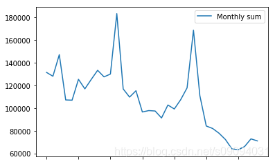
从上表中可以看出一共有21807件商品。使用sum()可以看到所有商品的总销量根据时间的变化关系。
sales_by_item_id.sum()[1:].plot(legend=True, label="Monthly sum")
<matplotlib.axes._subplots.AxesSubplot at 0x1e0806f0fd0>
分析有多少商品在最近的连续六个月内,没有销量。这些商品有多少出现在测试集中。
- 训练集一共21807种商品,其中有12391种在最近的六个月没有销量。
- 测试集一共5100种商品,其中有164种在训练中最近六个月没有销量,共出现了164 * 42 = 6888次。
- Tips:在最终的预测结果中,我们可以将这些商品的销量大胆地设置为零。
outdated_items = sales_by_item_id[sales_by_item_id.loc[:,'27':].sum(axis=1)==0]
print('Outdated items:', len(outdated_items))
test = pd.read_csv('../readonly/final_project_data/test.csv.gz')
print('unique items in test set:', test['item_id'].nunique())
print('Outdated items in test set:', test[test['item_id'].isin(outdated_items['item_id'])]['item_id'].nunique())
Outdated items: 12391
unique items in test set: 5100
Outdated items in test set: 164
在训练集种有6行,是重复出现的,我们可以删除或者保留,这种数据对结果影响不大。
print("duplicated lines in sales_train is", len(sales_train[sales_train.duplicated()]))
duplicated lines in sales_train is 6
2.1.2 每个商店的销量
一共有 60 个商店,坐落在31个城市,城市的信息可以作为商店的一个特征。
这里先分析下哪些商店是最近才开的,哪些是已经关闭了的,同样分析最后六个月的数据。
- shop_id = 36 是新商店
- shop_id = [0 1 8 11 13 17 23 29 30 32 33 40 43 54] 可以认为是已经关闭了。
- Tips:新商店,可以直接用第33个月来预测34个月的销量,因为它没有任何历史数据。而已经关闭的商店,销量可以直接置零
sales_by_shop_id = sales_train.pivot_table(index=['shop_id'],values=['item_cnt_day'],
                                        columns='date_block_num', aggfunc=np.sum, fill_value=0).reset_index()
sales_by_shop_id.columns = sales_by_shop_id.columns.droplevel().map(str)
sales_by_shop_id = sales_by_shop_id.reset_index(drop=True).rename_axis(None, axis=1)
sales_by_shop_id.columns.values[0] = 'shop_id'

for i in range(27,34):
    print('Not exists in month',i,sales_by_shop_id['shop_id'][sales_by_shop_id.loc[:,'0':str(i)].sum(axis=1)==0].unique())

for i in range(27,34):
    print('Shop is outdated for month',i,sales_by_shop_id['shop_id'][sales_by_shop_id.loc[:,str(i):].sum(axis=1)==0].unique())
Not exists in month 27 [36]
Not exists in month 28 [36]
Not exists in month 29 [36]
Not exists in month 30 [36]
Not exists in month 31 [36]
Not exists in month 32 [36]
Not exists in month 33 []
Shop is outdated for month 27 [ 0  1  8 11 13 17 23 30 32 40 43]
Shop is outdated for month 28 [ 0  1  8 11 13 17 23 30 32 33 40 43 54]
Shop is outdated for month 29 [ 0  1  8 11 13 17 23 29 30 32 33 40 43 54]
Shop is outdated for month 30 [ 0  1  8 11 13 17 23 29 30 32 33 40 43 54]
Shop is outdated for month 31 [ 0  1  8 11 13 17 23 29 30 32 33 40 43 54]
Shop is outdated for month 32 [ 0  1  8 11 13 17 23 29 30 32 33 40 43 54]
Shop is outdated for month 33 [ 0  1  8 11 13 17 23 27 29 30 32 33 40 43 51 54]
2.1.3 每类商品的销量
为了能使用商品的类别,需要先读取item_categories的信息,然后添加到sales_train里面
item_categories = pd.read_csv('../readonly/final_project_data/items.csv')
item_categories = item_categories[['item_id','item_category_id']]
item_categories.head()
| item_id | item_category_id | |
|---|---|---|
| 0 | 0 | 40 |
| 1 | 1 | 76 |
| 2 | 2 | 40 |
| 3 | 3 | 40 |
| 4 | 4 | 40 |
sales_train_merge_cat = pd.merge(sales_train,item_categories, on = 'item_id', how = 'left')
sales_train_merge_cat.head()
| date | date_block_num | shop_id | item_id | item_price | item_cnt_day | item_category_id | |
|---|---|---|---|---|---|---|---|
| 0 | 02.01.2013 | 0 | 59 | 22154 | 999.000000 | 1.0 | 37 |
| 1 | 03.01.2013 | 0 | 25 | 2552 | 899.000000 | 1.0 | 58 |
| 2 | 05.01.2013 | 0 | 25 | 2552 | 899.000000 | -1.0 | 58 |
| 3 | 06.01.2013 | 0 | 25 | 2554 | 1709.050049 | 1.0 | 58 |
| 4 | 15.01.2013 | 0 | 25 | 2555 | 1099.000000 | 1.0 | 56 |
2.1.4 销量和价格的离群值
从sales_train种找到销量和价格的离群值,然后删掉。
plt.figure(figsize=(10,4))
plt.xlim(-100,3000)
sns.boxplot(x = sales_train['item_cnt_day'])
print('Sale volume outliers:',sales_train['item_cnt_day'][sales_train['item_cnt_day']>1001].unique())
plt.figure(figsize=(10,4))
plt.xlim(-10000,320000)
sns.boxplot(x = sales_train['item_price'])
print('Sale price outliers:',sales_train['item_price'][sales_train['item_price']>300000].unique())
Sale volume outliers: [2169.]
Sale price outliers: [307980.]
sales_train = sales_train[sales_train['item_cnt_day'] <1001]
sales_train = sales_train[sales_train['item_price'] < 300000]
plt.figure(figsize=(10,4))
plt.xlim(-100,3000)
sns.boxplot(x = sales_train['item_cnt_day'])

plt.figure(figsize=(10,4))
plt.xlim(-10000,320000)
sns.boxplot(x = sales_train['item_price'])
<matplotlib.axes._subplots.AxesSubplot at 0x1e080864a20>


有一个商品的价格是负值,将其填充为median。
sales_train[sales_train['item_price']<0]
| date | date_block_num | shop_id | item_id | item_price | item_cnt_day | |
|---|---|---|---|---|---|---|
| 484683 | 15.05.2013 | 4 | 32 | 2973 | -1.0 | 1.0 |
median = sales_train[(sales_train['date_block_num'] == 4) & (sales_train['shop_id'] == 32)\
                     & (sales_train['item_id'] == 2973) & (sales_train['item_price']>0)].item_price.median()
sales_train.loc[sales_train['item_price']<0,'item_price'] = median
print(median)
1874.0
2.2 测试集分析
测试集有5100 种商品,42个商店。刚好就是5100 * 42 = 214200种 商品-商店组合。可以分为三大类
- 363种商品在训练集没有出现,363*42=15,246种商品-商店没有数据,约占7%。
- 87550种商品-商店组合是只出现过商品,没出现过组合。约占42%。
- 111404种商品-商店组合是在训练集中完整出现过的。约占51%。
test = pd.read_csv('../readonly/final_project_data/test.csv.gz')
good_sales = test.merge(sales_train, on=['item_id','shop_id'], how='left').dropna()
good_pairs = test[test['ID'].isin(good_sales['ID'])]
no_data_items = test[~(test['item_id'].isin(sales_train['item_id']))]

print('1. Number of good pairs:', len(good_pairs))
print('2. No Data Items:', len(no_data_items))
print('3. Only Item_id Info:', len(test)-len(no_data_items)-len(good_pairs))
1. Number of good pairs: 111404
2. No Data Items: 15246
3. Only Item_id Info: 87550
no_data_items.head()
| ID | shop_id | item_id | |
|---|---|---|---|
| 1 | 1 | 5 | 5320 |
| 4 | 4 | 5 | 5268 |
| 45 | 45 | 5 | 5826 |
| 64 | 64 | 5 | 3538 |
| 65 | 65 | 5 | 3571 |
2.3 商店特征
2.3.1 商店信息清洗
商店名里已经包含了很多特征,可以按以下结构分解。
城市 | 类型 | 名称
shops = pd.read_csv('../readonly/final_project_data/shops.csv')
shops.head()
| shop_name | shop_id | |
|---|---|---|
| 0 | !Якутск Орджоникидзе, 56 фран | 0 |
| 1 | !Якутск ТЦ "Центральный" фран | 1 |
| 2 | Адыгея ТЦ "Мега" | 2 |
| 3 | Балашиха ТРК "Октябрь-Киномир" | 3 |
| 4 | Волжский ТЦ "Волга Молл" | 4 |
经过分析,发现以下商店名为同一个商店,可以合并shop_id.
* 11 => 10
* 1 => 58
* 0 => 57
* 40 => 39
查看测试集,发现 shop id [0,1,11,40] 都不存在。
- shop_id = 0, 1 仅仅存在了两个月,而 shop_id = 57,58 看起来就像是继任者。
- shop_id = 11 仅仅存在于 date_block = 25,而 shop_id = 10 只在那个月没有数据。
- shop_id = 40 仅仅存在于 date_block = [14,25] 而 shop_id = 39 在 date_block = 14 之后一直存在。
- shop_id = 46,商店名中间多了一个空格,会影响到编码,要去掉。 Сергиев Посад ТЦ “7Я”
- 通过商店命名,我发现shop 12 and 55都是网店,并且发现他们的销量的相关度很高,只是不知道怎么用这个信息。
sales12 = np.array(sales_by_shop_id.loc[sales_by_shop_id['shop_id'] == 12 ].values)
sales12 = sales12[:,1:].reshape(-1)
sales55 = np.array(sales_by_shop_id.loc[sales_by_shop_id['shop_id'] == 55 ].values)
sales55 = sales55[:,1:].reshape(-1)
months = np.array(sales_by_shop_id.loc[sales_by_shop_id['shop_id'] == 12 ].columns[1:])
np.corrcoef(sales12,sales55)
array([[1.        , 0.69647514],
       [0.69647514, 1.        ]])
test.shop_id.sort_values().unique()
array([ 2,  3,  4,  5,  6,  7, 10, 12, 14, 15, 16, 18, 19, 21, 22, 24, 25,
       26, 28, 31, 34, 35, 36, 37, 38, 39, 41, 42, 44, 45, 46, 47, 48, 49,
       50, 52, 53, 55, 56, 57, 58, 59], dtype=int64)
sales_train.loc[sales_train['shop_id'] == 0,'shop_id'] = 57
sales_train.loc[sales_train['shop_id'] == 1,'shop_id'] = 58
sales_train.loc[sales_train['shop_id'] == 11,'shop_id'] = 10
sales_train.loc[sales_train['shop_id'] == 40,'shop_id'] = 39
2.3.2 商店信息编码
shops['shop_name'] = shops['shop_name'].apply(lambda x: x.lower()).str.replace('[^\w\s]', '').str.replace('\d+','').str.strip()
shops['shop_city'] = shops['shop_name'].str.partition(' ')[0]
shops['shop_type'] = shops['shop_name'].apply(lambda x: 'мтрц' if 'мтрц' in x else 'трц' if 'трц' in x else 'трк' if 'трк' in x else 'тц' if 'тц' in x else 'тк' if 'тк' in x else 'NO_DATA')
shops.head()
| shop_name | shop_id | shop_city | shop_type | |
|---|---|---|---|---|
| 0 | якутск орджоникидзе фран | 0 | якутск | NO_DATA |
| 1 | якутск тц центральный фран | 1 | якутск | тц |
| 2 | адыгея тц мега | 2 | адыгея | тц |
| 3 | балашиха трк октябрькиномир | 3 | балашиха | трк |
| 4 | волжский тц волга молл | 4 | волжский | тц |
shops['shop_city_code'] = LabelEncoder().fit_transform(shops['shop_city'])
shops['shop_type_code'] = LabelEncoder().fit_transform(shops['shop_type'])
shops.head()
| shop_name | shop_id | shop_city | shop_type | shop_city_code | shop_type_code | |
|---|---|---|---|---|---|---|
| 0 | якутск орджоникидзе фран | 0 | якутск | NO_DATA | 29 | 0 |
| 1 | якутск тц центральный фран | 1 | якутск | тц | 29 | 5 |
| 2 | адыгея тц мега | 2 | адыгея | тц | 0 | 5 |
| 3 | балашиха трк октябрькиномир | 3 | балашиха | трк | 1 | 3 |
| 4 | волжский тц волга молл | 4 | волжский | тц | 2 | 5 |
2.4 商品分类特征
商品类别之间的距离不好确定,使用one hot编码更加合适。
categories = pd.read_csv('../readonly/final_project_data/item_categories.csv')
lines1 = [26,27,28,29,30,31]
lines2 = [81,82]
for index in lines1:
    category_name = categories.loc[index,'item_category_name']
#    print(category_name)
    category_name = category_name.replace('Игры','Игры -')
#    print(category_name)
    categories.loc[index,'item_category_name'] = category_name
for index in lines2:
    category_name = categories.loc[index,'item_category_name']
#    print(category_name)
    category_name = category_name.replace('Чистые','Чистые -')
#    print(category_name)
    categories.loc[index,'item_category_name'] = category_name
category_name = categories.loc[32,'item_category_name']
#print(category_name)
category_name = category_name.replace('Карты оплаты','Карты оплаты -')
#print(category_name)
categories.loc[32,'item_category_name'] = category_name
categories.head()
| item_category_name | item_category_id | |
|---|---|---|
| 0 | PC - Гарнитуры/Наушники | 0 |
| 1 | Аксессуары - PS2 | 1 |
| 2 | Аксессуары - PS3 | 2 |
| 3 | Аксессуары - PS4 | 3 |
| 4 | Аксессуары - PSP | 4 |
categories['split'] = categories['item_category_name'].str.split('-')
categories['type'] = categories['split'].map(lambda x:x[0].strip())
categories['subtype'] = categories['split'].map(lambda x:x[1].strip() if len(x)>1 else x[0].strip())
categories = categories[['item_category_id','type','subtype']]
categories.head()
| item_category_id | type | subtype | |
|---|---|---|---|
| 0 | 0 | PC | Гарнитуры/Наушники |
| 1 | 1 | Аксессуары | PS2 |
| 2 | 2 | Аксессуары | PS3 |
| 3 | 3 | Аксессуары | PS4 |
| 4 | 4 | Аксессуары | PSP |
categories['cat_type_code'] = LabelEncoder().fit_transform(categories['type'])
categories['cat_subtype_code'] = LabelEncoder().fit_transform(categories['subtype'])
categories.head()
| item_category_id | type | subtype | cat_type_code | cat_subtype_code | |
|---|---|---|---|---|---|
| 0 | 0 | PC | Гарнитуры/Наушники | 0 | 33 |
| 1 | 1 | Аксессуары | PS2 | 1 | 13 |
| 2 | 2 | Аксессуары | PS3 | 1 | 14 |
| 3 | 3 | Аксессуары | PS4 | 1 | 15 |
| 4 | 4 | Аксессуары | PSP | 1 | 17 |
3 特征融合
3.1 统计月销量
首先将训练集中的数据统计好月销量
ts = time.time()
matrix = []
cols = ['date_block_num','shop_id','item_id']
for i in range(34):
    sales = sales_train[sales_train.date_block_num==i]
    matrix.append(np.array(list(product([i], sales.shop_id.unique(), sales.item_id.unique())), dtype='int16'))

matrix = pd.DataFrame(np.vstack(matrix), columns=cols)
matrix['date_block_num'] = matrix['date_block_num'].astype(np.int8)
matrix['shop_id'] = matrix['shop_id'].astype(np.int8)
matrix['item_id'] = matrix['item_id'].astype(np.int16)
matrix.sort_values(cols,inplace=True)
time.time() - ts

sales_train['revenue'] = sales_train['item_price'] *  sales_train['item_cnt_day']

groupby = sales_train.groupby(['item_id','shop_id','date_block_num']).agg({'item_cnt_day':'sum'})
groupby.columns = ['item_cnt_month']
groupby.reset_index(inplace=True)
matrix = matrix.merge(groupby, on = ['item_id','shop_id','date_block_num'], how = 'left')
matrix['item_cnt_month'] = matrix['item_cnt_month'].fillna(0).clip(0,20).astype(np.float16)
matrix.head()

test['date_block_num'] = 34
test['date_block_num'] = test['date_block_num'].astype(np.int8)
test['shop_id'] = test['shop_id'].astype(np.int8)
test['item_id'] = test['item_id'].astype(np.int16)
test.shape

cols = ['date_block_num','shop_id','item_id']
matrix = pd.concat([matrix, test[['item_id','shop_id','date_block_num']]], ignore_index=True, sort=False, keys=cols)
matrix.fillna(0, inplace=True) # 34 month
print(matrix.head())
   date_block_num  shop_id  item_id  item_cnt_month
0               0        2       19             0.0
1               0        2       27             1.0
2               0        2       28             0.0
3               0        2       29             0.0
4               0        2       32             0.0
这里要确保矩阵里面没有 NA和NULL
print(matrix['item_cnt_month'].isna().sum())
print(matrix['item_cnt_month'].isnull().sum())
0
0
3.2 相关信息融合
将上面得到的商店,商品类别等信息与矩阵融合起来。
ts = time.time()
matrix = matrix.merge(items[['item_id','item_category_id']], on = ['item_id'], how = 'left')
matrix = matrix.merge(categories[['item_category_id','cat_type_code','cat_subtype_code']], on = ['item_category_id'], how = 'left')
matrix = matrix.merge(shops[['shop_id','shop_city_code','shop_type_code']], on = ['shop_id'], how = 'left')
matrix['shop_city_code'] = matrix['shop_city_code'].astype(np.int8)
matrix['shop_type_code'] = matrix['shop_type_code'].astype(np.int8)
matrix['item_category_id'] = matrix['item_category_id'].astype(np.int8)
matrix['cat_type_code'] = matrix['cat_type_code'].astype(np.int8)
matrix['cat_subtype_code'] = matrix['cat_subtype_code'].astype(np.int8)
time.time() - ts
4.71001935005188
matrix.head()
| date_block_num | shop_id | item_id | item_cnt_month | item_category_id | cat_type_code | cat_subtype_code | shop_city_code | shop_type_code | |
|---|---|---|---|---|---|---|---|---|---|
| 0 | 0 | 2 | 19 | 0.0 | 40 | 7 | 6 | 0 | 5 |
| 1 | 0 | 2 | 27 | 1.0 | 19 | 5 | 14 | 0 | 5 |
| 2 | 0 | 2 | 28 | 0.0 | 30 | 5 | 12 | 0 | 5 |
| 3 | 0 | 2 | 29 | 0.0 | 23 | 5 | 20 | 0 | 5 |
| 4 | 0 | 2 | 32 | 0.0 | 40 | 7 | 6 | 0 | 5 |
matrix.info()
<class 'pandas.core.frame.DataFrame'>
Int64Index: 11056140 entries, 0 to 11056139
Data columns (total 9 columns):
date_block_num      int8
shop_id             int8
item_id             int16
item_cnt_month      float16
item_category_id    int8
cat_type_code       int8
cat_subtype_code    int8
shop_city_code      int8
shop_type_code      int8
dtypes: float16(1), int16(1), int8(7)
memory usage: 200.3 MB
3.2 历史信息
将产生的信息做了融合。需要通过延迟操作来产生一些历史信息。比如可以将第0-33个月的销量作为第1-34个月的历史特征(延迟一个月)。按照以下说明,一共产生了15种特征。
- 每个商品-商店组合每个月销量的历史信息,分别延迟[1,2,3,6,12]个月。这应该是最符合直觉的一种操作。
- 所有商品-商店组合每个月销量均值的历史信息,分别延迟[1,2,3,6,12]个月。
- 每件商品每个月销量均值的历史信息,分别延迟[1,2,3,6,12]个月。
- 每个商店每个月销量均值的历史信息,分别延迟[1,2,3,6,12]个月。
- 每个商品类别每个月销量均值的历史信息,分别延迟[1,2,3,6,12]个月。
- 每个商品类别-商店每个月销量均值的历史信息,分别延迟[1,2,3,6,12]个月。
以上六种延迟都比较直观,直接针对商品,商店,商品类别。但是销量的变化趋势还可能与商品类别_大类,商店_城市,商品价格,每个月的天数有关,还需要做以下统计和延迟。可以根据模型输出的feature importance来选择和调整这些特征。
- 每个商品类别_大类每个月销量均值的历史信息,分别延迟[1,2,3,6,12]个月。
- 每个商店_城市每个月销量均值的历史信息,分别延迟[1,2,3,6,12]个月。
- 每个商品-商店_城市组合每个月销量均值的历史信息,分别延迟[1,2,3,6,12]个月。
除了以上组合之外,还有以下特征可能有用
- 每个商品第一次的销量
- 每个商品最后一次的销量
- 每个商品_商店组合第一次的销量
- 每个商品_商店组合最后一次的销量
- 每个商品的价格变化
- 每个月的天数
3.2.1 lag operation产生延迟信息,可以选择延迟的月数。
def lag_feature(df, lags, col):
    tmp = df[['date_block_num','shop_id','item_id',col]]
    for i in lags:
        shifted = tmp.copy()
        shifted.columns = ['date_block_num','shop_id','item_id', col+'_lag_'+str(i)]
        shifted['date_block_num'] += i
        df = pd.merge(df, shifted, on=['date_block_num','shop_id','item_id'], how='left')
    return df
3.2.2 月销量(每个商品-商店)的历史信息
针对每个月的商品-商店组合的销量求一个历史信息,分别是1个月、2个月、3个月、6个月、12个月前的销量。这个值和我们要预测的值是同一个数量级,不需要求平均。而且会有很多值会是NAN,因为不存在这样的历史信息,具体原因前面已经分析过。
ts = time.time()
matrix = lag_feature(matrix, [1,2,3,6,12], 'item_cnt_month')
time.time() - ts
27.62108063697815
3.2.3 月销量(所有商品-商店)均值的历史信息
统计每个月的销量,这里的销量是包括了该月的所有商品-商店组合,所以需要求平均。同求历史信息。
ts = time.time()
group = matrix.groupby(['date_block_num']).agg({'item_cnt_month': ['mean']})
group.columns = [ 'date_avg_item_cnt' ]
group.reset_index(inplace=True)

matrix = pd.merge(matrix, group, on=['date_block_num'], how='left')
matrix['date_avg_item_cnt'] = matrix['date_avg_item_cnt'].astype(np.float16)
matrix = lag_feature(matrix, [1,2,3,6,12], 'date_avg_item_cnt')
matrix.drop(['date_avg_item_cnt'], axis=1, inplace=True)
time.time() - ts
33.013164043426514
3.2.4 月销量(每件商品)均值和历史特征
统计每件商品在每个月的销量,这里的销量是包括了该月该商品在所有商店的销量,所以需要求平均。同求历史信息。
ts = time.time()
group = matrix.groupby(['date_block_num', 'item_id']).agg({'item_cnt_month': ['mean']})
group.columns = [ 'date_item_avg_item_cnt' ]
group.reset_index(inplace=True)

matrix = pd.merge(matrix, group, on=['date_block_num','item_id'], how='left')
matrix['date_item_avg_item_cnt'] = matrix['date_item_avg_item_cnt'].astype(np.float16)
matrix = lag_feature(matrix, [1,2,3,6,12], 'date_item_avg_item_cnt')
matrix.drop(['date_item_avg_item_cnt'], axis=1, inplace=True)
time.time() - ts
3.2.5 月销量(每个商店)均值和历史特征
统计每个商店在每个月的销量,这里的销量是包括了该月该商店的所有商品的销量,所以需要求平均。同求历史信息。
ts = time.time()
group = matrix.groupby(['date_block_num', 'shop_id']).agg({'item_cnt_month': ['mean']})
group.columns = [ 'date_shop_avg_item_cnt' ]
group.reset_index(inplace=True)

matrix = pd.merge(matrix, group, on=['date_block_num','shop_id'], how='left')
matrix['date_shop_avg_item_cnt'] = matrix['date_shop_avg_item_cnt'].astype(np.float16)
matrix = lag_feature(matrix, [1,2,3,6,12], 'date_shop_avg_item_cnt')
matrix.drop(['date_shop_avg_item_cnt'], axis=1, inplace=True)
time.time() - ts
3.2.6 月销量(每个商品类别)均值和历史特征
统计每个商品类别在每个月的销量,这里的销量是包括了该月该商品类别的所有销量,所以需要求平均。同求历史信息。
ts = time.time()
group = matrix.groupby(['date_block_num', 'item_category_id']).agg({'item_cnt_month': ['mean']})
group.columns = [ 'date_cat_avg_item_cnt' ]
group.reset_index(inplace=True)

matrix = pd.merge(matrix, group, on=['date_block_num','item_category_id'], how='left')
matrix['date_cat_avg_item_cnt'] = matrix['date_cat_avg_item_cnt'].astype(np.float16)
matrix = lag_feature(matrix, [1,2,3,6,12], 'date_cat_avg_item_cnt')
matrix.drop(['date_cat_avg_item_cnt'], axis=1, inplace=True)
time.time() - ts
3.2.7 月销量(商品类别-商店)均值和历史特征
统计每个商品类别-商店在每个月的销量,这里的销量是包括了该月该商品商店_城市的所有销量,所以需要求平均。同求历史信息。
ts = time.time()
group = matrix.groupby(['date_block_num', 'item_category_id','shop_id']).agg({'item_cnt_month': ['mean']})
group.columns = [ 'date_cat_shop_avg_item_cnt' ]
group.reset_index(inplace=True)

matrix = pd.merge(matrix, group, on=['date_block_num', 'item_category_id','shop_id'], how='left')
matrix['date_cat_shop_avg_item_cnt'] = matrix['date_cat_shop_avg_item_cnt'].astype(np.float16)
matrix = lag_feature(matrix, [1,2,3,6,12], 'date_cat_shop_avg_item_cnt')
matrix.drop(['date_cat_shop_avg_item_cnt'], axis=1, inplace=True)
time.time() - ts
15.178605556488037
matrix.info()
3.2.8 月销量(商品类别_大类)均值和历史特征
统计每个商品类别_大类在每个月的销量,这里的销量是包括了该月该商品类别_大类的所有销量,所以需要求平均。同求历史信息。
ts = time.time()
group = matrix.groupby(['date_block_num', 'cat_type_code']).agg({'item_cnt_month': ['mean']})
group.columns = [ 'date_type_avg_item_cnt' ]
group.reset_index(inplace=True)

matrix = pd.merge(matrix, group, on=['date_block_num','cat_type_code'], how='left')
matrix['date_type_avg_item_cnt'] = matrix['date_type_avg_item_cnt'].astype(np.float16)
matrix = lag_feature(matrix, [1,2,3,6,12], 'date_type_avg_item_cnt')
matrix.drop(['date_type_avg_item_cnt'], axis=1, inplace=True)
time.time() - ts
14.34829592704773
3.2.9 月销量(商品-商品类别_大类)均值和历史特征
ts = time.time()
group = matrix.groupby(['date_block_num', 'item_id','cat_type_code']).agg({'item_cnt_month': ['mean']})
group.columns = [ 'date_item_type_avg_item_cnt' ]
group.reset_index(inplace=True)

matrix = pd.merge(matrix, group, on=['date_block_num','item_id','cat_type_code'], how='left')
matrix['date_item_type_avg_item_cnt'] = matrix['date_item_type_avg_item_cnt'].astype(np.float16)
matrix = lag_feature(matrix, [1,2,3,6,12], 'date_item_type_avg_item_cnt')
matrix.drop(['date_item_type_avg_item_cnt'], axis=1, inplace=True)
time.time() - ts
14.34829592704773
3.2.10 月销量(商店_城市)均值和历史特征
统计每个商店_城市在每个月的销量,这里的销量是包括了该月该商店_城市的所有销量,所以需要求平均。同求历史信息。
ts = time.time()
group = matrix.groupby(['date_block_num', 'shop_city_code']).agg({'item_cnt_month': ['mean']})
group.columns = ['date_city_avg_item_cnt']
group.reset_index(inplace=True)

matrix = pd.merge(matrix, group, on=['date_block_num',  'shop_city_code'], how='left')
matrix['date_city_avg_item_cnt'] = matrix['date_city_avg_item_cnt'].astype(np.float16)
matrix = lag_feature(matrix, [1,2,3,6,12], 'date_city_avg_item_cnt')
matrix.drop(['date_city_avg_item_cnt'], axis=1, inplace=True)
time.time() - ts
14.687093496322632
3.2.11 月销量(商品-商店_城市)均值和历史特征
统计每个商品-商店_城市在每个月的销量,这里的销量是包括了该月该商品-商店_城市的所有销量,所以需要求平均。同求历史信息。
ts = time.time()
group = matrix.groupby(['date_block_num','item_id', 'shop_city_code']).agg({'item_cnt_month': ['mean']})
group.columns = ['date_item_city_avg_item_cnt']
group.reset_index(inplace=True)

matrix = pd.merge(matrix, group, on=['date_block_num', 'item_id', 'shop_city_code'], how='left')
matrix['date_item_city_avg_item_cnt'] = matrix['date_item_city_avg_item_cnt'].astype(np.float16)
matrix = lag_feature(matrix, [1,2,3,6,12], 'date_item_city_avg_item_cnt')
matrix.drop(['date_item_city_avg_item_cnt'], axis=1, inplace=True)
time.time() - ts
14.687093496322632
3.2.12 趋势特征,半年来价格的变化
ts = time.time()
group = sales_train.groupby(['item_id']).agg({'item_price': ['mean']})
group.columns = ['item_avg_item_price']
group.reset_index(inplace=True)

matrix = pd.merge(matrix, group, on=['item_id'], how='left')
matrix['item_avg_item_price'] = matrix['item_avg_item_price'].astype(np.float16)

group = sales_train.groupby(['date_block_num','item_id']).agg({'item_price': ['mean']})
group.columns = ['date_item_avg_item_price']
group.reset_index(inplace=True)

matrix = pd.merge(matrix, group, on=['date_block_num','item_id'], how='left')
matrix['date_item_avg_item_price'] = matrix['date_item_avg_item_price'].astype(np.float16)

lags = [1,2,3,4,5,6,12]
matrix = lag_feature(matrix, lags, 'date_item_avg_item_price')

for i in lags:
    matrix['delta_price_lag_'+str(i)] = \
        (matrix['date_item_avg_item_price_lag_'+str(i)] - matrix['item_avg_item_price']) / matrix['item_avg_item_price']

def select_trend(row):
    for i in lags:
        if row['delta_price_lag_'+str(i)]:
            return row['delta_price_lag_'+str(i)]
    return 0

matrix['delta_price_lag'] = matrix.apply(select_trend, axis=1)
matrix['delta_price_lag'] = matrix['delta_price_lag'].astype(np.float16)
matrix['delta_price_lag'].fillna(0, inplace=True)

# https://stackoverflow.com/questions/31828240/first-non-null-value-per-row-from-a-list-of-pandas-columns/31828559
# matrix['price_trend'] = matrix[['delta_price_lag_1','delta_price_lag_2','delta_price_lag_3']].bfill(axis=1).iloc[:, 0]
# Invalid dtype for backfill_2d [float16]

fetures_to_drop = ['item_avg_item_price', 'date_item_avg_item_price']
for i in lags:
    fetures_to_drop += ['date_item_avg_item_price_lag_'+str(i)]
    fetures_to_drop += ['delta_price_lag_'+str(i)]

matrix.drop(fetures_to_drop, axis=1, inplace=True)

time.time() - ts
601.2605240345001
3.2.13 每个月天数
matrix['month'] = matrix['date_block_num'] % 12
days = pd.Series([31,28,31,30,31,30,31,31,30,31,30,31])
matrix['days'] = matrix['month'].map(days).astype(np.int8)
3.2.14 开始和结束的销量
Months since the last sale for each shop/item pair and for item only. I use programing approach.
Create HashTable with key equals to {shop_id,item_id} and value equals to date_block_num. Iterate data from the top. Foreach row if {row.shop_id,row.item_id} is not present in the table, then add it to the table and set its value to row.date_block_num. if HashTable contains key, then calculate the difference beteween cached value and row.date_block_num.
ts = time.time()
cache = {}
matrix['item_shop_last_sale'] = -1
matrix['item_shop_last_sale'] = matrix['item_shop_last_sale'].astype(np.int8)
for idx, row in matrix.iterrows():
    key = str(row.item_id)+' '+str(row.shop_id)
    if key not in cache:
        if row.item_cnt_month!=0:
            cache[key] = row.date_block_num
    else:
        last_date_block_num = cache[key]
        matrix.at[idx, 'item_shop_last_sale'] = row.date_block_num - last_date_block_num
        cache[key] = row.date_block_num
time.time() - ts
Months since the first sale for each shop/item pair and for item only.
ts = time.time()
matrix['item_shop_first_sale'] = matrix['date_block_num'] - matrix.groupby(['item_id','shop_id'])['date_block_num'].transform('min')
matrix['item_first_sale'] = matrix['date_block_num'] - matrix.groupby('item_id')['date_block_num'].transform('min')
time.time() - ts
2.4333603382110596
因为使用了12个月作为延迟特征,必然由大量的数据是NA值,将最开始11个月的原始特征删除,并且对于NA值我们需要把它填充为0。
ts = time.time()
matrix = matrix[matrix.date_block_num > 11]
time.time() - ts
1.0133898258209229
ts = time.time()
def fill_na(df):
    for col in df.columns:
        if ('_lag_' in col) & (df[col].isnull().any()):
            if ('item_cnt' in col):
                df[col].fillna(0, inplace=True)
    return df

matrix = fill_na(matrix)
time.time() - ts
4. 数据建模
4.1 lightgbm 模型
import numpy as np
import pandas as pd
import matplotlib.pyplot as plt
import seaborn as sns
import time
import gc
import pickle
from itertools import product
from sklearn.preprocessing import LabelEncoder

pd.set_option('display.max_rows', 500)
pd.set_option('display.max_columns', 100)

#import sklearn.model_selection.KFold as KFold
def plot_features(booster, figsize):
    fig, ax = plt.subplots(1,1,figsize=figsize)
    return plot_importance(booster=booster, ax=ax)
data = pd.read_pickle('data_simple.pkl')
X_train = data[data.date_block_num < 33].drop(['item_cnt_month'], axis=1)
Y_train = data[data.date_block_num < 33]['item_cnt_month']
X_valid = data[data.date_block_num == 33].drop(['item_cnt_month'], axis=1)
Y_valid = data[data.date_block_num == 33]['item_cnt_month']
X_test = data[data.date_block_num == 34].drop(['item_cnt_month'], axis=1)
del data
gc.collect();
import lightgbm as lgb

ts = time.time()
train_data = lgb.Dataset(data=X_train, label=Y_train)
valid_data = lgb.Dataset(data=X_valid, label=Y_valid)

time.time() - ts

params = {"objective" : "regression", "metric" : "rmse", 'n_estimators':10000, 'early_stopping_rounds':50,
              "num_leaves" : 200, "learning_rate" : 0.01, "bagging_fraction" : 0.9,
              "feature_fraction" : 0.3, "bagging_seed" : 0}

lgb_model = lgb.train(params, train_data, valid_sets=[train_data, valid_data], verbose_eval=1000)
Y_test = lgb_model.predict(X_test).clip(0, 20)
I want to change some values to be zeros.
4.2. 后处理
4.2.1 过期商品
将最近12个月都没有销售的商品的销量置零。
4.3 重要性画图


 3661
3661

 被折叠的 条评论
为什么被折叠?
被折叠的 条评论
为什么被折叠?
 到【灌水乐园】发言


