02_逻辑回归

线性可分数据→逻辑回归
非线性可分数据→多项式逻辑回归
多分类问题→OvO， OvR

1 逻辑回归代码实现

import numpy as np
import matplotlib.pyplot as plt
from sklearn.model_selection import train_test_split
from sklearn.datasets import make_classification
from sklearn.linear_model import LogisticRegression

x, y = make_classification(
    n_samples=200,
    n_features=2,
    n_redundant=0,
    n_classes=2,
    n_clusters_per_class=1,
    random_state=50
)
print(x.shape, y.shape)
x_train, x_test, y_train, y_test = train_test_split(x, y, train_size=0.7, random_state=0, stratify=y)
plt.scatter(x_train[:, 0], x_train[:, 1], c=y_train)
plt.show()

clf = LogisticRegression()
clf.fit(x_train, y_train)
print(clf.score(x_train, y_train))
print(clf.score(x_test, y_test))
y_predict = clf.predict(x_test)
print(y_predict)
print(clf.predict_proba(x_test)[:3])
print(np.argmax(clf.predict_proba(x_test), axis=1))

(200, 2) (200,)
0.9571428571428572
0.9666666666666667
[0 1 0 1 0 0 0 1 1 1 0 1 0 0 0 1 1 0 0 0 1 1 0 1 1 0 1 1 0 1 1 0 0 0 1 0 1
0 0 0 1 1 1 0 1 1 0 1 0 0 1 0 1 0 0 1 1 0 0 0]
[[0.9976049 0.0023951 ]
[0.00943605 0.99056395]
[0.99884752 0.00115248]]
[0 1 0 1 0 0 0 1 1 1 0 1 0 0 0 1 1 0 0 0 1 1 0 1 1 0 1 1 0 1 1 0 0 0 1 0 1
0 0 0 1 1 1 0 1 1 0 1 0 0 1 0 1 0 0 1 1 0 0 0]

2 超参数

from sklearn.model_selection import train_test_split
from sklearn.datasets import make_classification
from sklearn.linear_model import LogisticRegression
from sklearn.model_selection import GridSearchCV

x, y = make_classification(
    n_samples=200,
    n_features=2,
    n_redundant=0,
    n_classes=2,
    n_clusters_per_class=1,
    random_state=50
)
print(x.shape, y.shape)
x_train, x_test, y_train, y_test = train_test_split(x, y, train_size=0.7, random_state=0, stratify=y)

params = [{
    'penalty': ['l2', 'l1'],
    'C': [0.0001, 0.001, 0.01, 0.1, 1, 10, 100, 1000],
    'solver': ['liblinear']
}, {
    'penalty': ['none'],
    'C': [0.0001, 0.001, 0.01, 0.1, 1, 10, 100, 1000],
    'solver': ['lbfgs']
}, {
    'penalty': ['elasticnet'],
    'C': [0.0001, 0.001, 0.01, 0.1, 1, 10, 100, 1000],
    'l1_ratio': [0, 0.25, 0.5, 0.75, 1],
    'solver': ['saga'],
    'max_iter': [200]
}]
grid = GridSearchCV(
    estimator=LogisticRegression(),
    param_grid=params,
    n_jobs=-1
)
grid.fit(x_train, y_train)
print(grid.best_score_)
print(grid.best_estimator_.score(x_test, y_test))
print(grid.best_params_)

0.9571428571428573
0.9666666666666667
{‘C’: 1, ‘penalty’: ‘l2’, ‘solver’: ‘liblinear’}

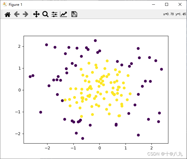
3 多项式逻辑回归

import numpy as np
import matplotlib.pyplot as plt
from sklearn.model_selection import train_test_split
from sklearn.linear_model import LogisticRegression
from sklearn.preprocessing import PolynomialFeatures

np.random.seed(0)
X = np.random.normal(0, 1, size=(200, 2))
y = np.array((X[:, 0] ** 2) + (X[:, 1] ** 2) < 2, dtype='int')
x_train, x_test, y_train, y_test = train_test_split(X, y, train_size=0.7, random_state=233, stratify=y)
plt.scatter(x_train[:,0], x_train[:,1], c = y_train)
plt.show()

clf = LogisticRegression()
clf.fit(x_train, y_train)
print(clf.score(x_train, y_train))
print(clf.score(x_train, y_train))

# 采用多项式逻辑回归
print('------采用多项式逻辑回归--------')
poly = PolynomialFeatures(degree=2)
poly.fit(x_train)
x2 = poly.transform(x_train)
x2t = poly.transform(x_test)
clf.fit(x2, y_train)
print(clf.score(x2, y_train))
print(clf.score(x2t, y_test))

0.7071428571428572
0.7071428571428572
------采用多项式逻辑回归--------
1.0
0.9666666666666667

4 多分类

from sklearn import datasets
from sklearn.linear_model import LogisticRegression
from sklearn.model_selection import train_test_split
from sklearn.multiclass import OneVsRestClassifier
from sklearn.multiclass import OneVsOneClassifier

iris = datasets.load_iris()
x = iris.data
y = iris.target
x_train, x_test, y_train, y_test = train_test_split(x, y, random_state=30)
clf = LogisticRegression()
ovr = OneVsRestClassifier(clf)
ovr.fit(x_train, y_train)
print("ovr.score:")
print(ovr.score(x_test, y_test))

ovr = OneVsOneClassifier(clf)
ovr.fit(x_train, y_train)
print("ovo.score:")
print(ovr.score(x_test, y_test))

ovr.score:
0.9473684210526315
ovo.score:
1.0