


softmax分类
对数几率回归解决的是二分类的问题,对于多个选项的问题,我们可以使用softmax函数,它是对数几率回归在 N 个可能不同的值上的推广。
神经网络的原始输出不是一个概率值,实质上只是输入的数值做了复杂的加权和与非线性处理之后的一个值而已,那么如何将这个输出变为概率分布?这就得看softmax层了。

softmax要求每个样本必须属于某个类别,且所有可能的样本均被覆盖 。
softmax会输出这个样本属于某一个类别的概率,假如有三个类别,对于每一个样本,他就会输出一个长度为三的张量,在这个长度为3的张量上,它的每一个位置都标志这个样本属于这一类的概率。比如说第一类是0.1,第二类是0.4,第三类是0.5; 这三个类别的概率相加为1。这样就把每一个类别都覆盖到了。
softmax个样本分量之和为 1,相当于逻辑回归在多个分类上的推广 ;当只有两个类别时,与对数几率回归完全相同。
熵在信息论中代表随机变量不确定度的度量。熵越大,数据的不确定性就越高;熵越小,数据的不确定性越低。
在 pytorch 里,对于多分类问题我们使用nn.CrossEntropyLoss() 和nn.NLLLoss等来计算 softmax 交叉熵。
这里交叉熵实际上就是 两个概率分布的之间距离的度量;比如说,模型输出的是[0.1 0.7 0.2],实际上是[0 0 1],我们就可以使用nn.CrossEntropyLoss计算这两个概率分布之间的损失。
鸢尾花数据集
数据预处理
import torch
import pandas as pd
import numpy as np
import matplotlib.pyplot as plt

data = pd.read_csv('../daatset/iris.csv')
data.head()
data.Species.unique() # 三分类问题 
Species列是我们要预测的结果,这个结果是一个字符串类型,我们需要把它转换成数值类型。 使用pandas的 方法将它编码成0、1、2、3、4...的形式
pd.factorize(data.Species) # 因为Species是字符形式,所以要将Species编码成0、1、2的形式。返回值是一个元祖,第一部分是转换后的array,第二部分是对应类别的名称
pd.factorize(data.Species)[0]
data['Species'] = pd.factorize(data.Species)[0]
ata[0:100:3]
# 可以看到Species列已经转化为了数值类型 
# iloc按位置取值
X = data.iloc[:,1:-1].values #第0列是序号,我们不要,使用 .values 将其转换为ndarray形式
# Y = data.Species.values.reshape(-1,1)
Y = data.Species.values

print('X.shape:',X.shape)
print('Y.shape:',Y.shape) 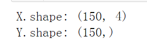
划分数据集
from sklearn.model_selection import train_test_split

train_X,test_X,train_Y,test_Y = train_test_split(X,Y)

# 出现报错,RuntimeError:expected scaler type Long but found Float
# 这是,我们希望目标的数据类型是long tensor(int tensor),而不是float tensor。
# 目标值是0、1、2这种形式,要求是一个long tensor,64位的整形。

# ndarray转换为tensor
train_X = torch.from_numpy(train_X).type(torch.float32)
# train_Y = torch.from_numpy(train_Y).type(torch.float32)
train_Y = torch.from_numpy(train_Y).type(torch.int64)

test_X = torch.from_numpy(test_X).type(torch.float32)
# test_Y = torch.from_numpy(test_Y).type(torch.float32)
test_Y = torch.from_numpy(test_Y).type(torch.LongTensor)
包装张量
rom torch.utils.data import TensorDataset
from torch.utils.data import DataLoader

batch = 8 #批次大小

train_ds = TensorDataset(train_X,train_Y) # Dataset
train_dl = DataLoader(train_ds,batch_size=batch,shuffle=True) # DataLoader

test_ds = TensorDataset(test_X,test_Y)
test_dl = DataLoader(test_ds,batch_size=batch) # 对于测试数据没有必要做shuffle
创建模型
import torch.nn.functional as F
from torch import nn

class Model(nn.Module):
    def __init__(self):

        #首先要继承父类中所有的变量
        super().__init__()

        # 开始初始化所有的层
        self.linear1 = nn.Linear(4,32 ) # 第一个线性层。将输入的4个特征输出到64个特征的隐藏层。
        self.linear2 = nn.Linear(32,32)
        self.linear3 = nn.Linear(32,3)  # 输出层。因为是三分类,所以输出特征长度为3。

    def forward(self,input):
        # forward方法有一个input参数,你的输入是交给forward方法,然后forward方法调用这些层对输入数据处理。

        # 线性层1,4 ---> 32
        x1 = F.relu(self.linear1(input))

        # 线性层2,32 ---> 32
        x2 =  F.relu(self.linear2(x1))

        # 输出层,32 ----> 3
#         x3 = F.sigmoid(self.linear3(x2)) # 用这个会有警告
#         x3 = torch.sigmoid(self.linear3(x2))
        x3 = self.linear3(x2)

        return x3
"""
在输出层,我们不进行激活,因为我们这个是三分类,使用的损失函数是CrossEntropyLoss,它的输入是一个未激活的输出。
它会在函数内部进行一次 ...softmax 进行计算,然后与我们真实的概率分布计算一个损失。
所以在这里面是不需要对预测结果进行激活的。
如果不对预测结果进行激活,一样可以得到输出,使用softmax只是把它映射到了一个长度为1的概率分布上。
如果不激活,输出结果最大的值仍然是概率分布最高的值,也就是肯输出[1,50,2],虽然没有经过softmax进行激活,
但是它最大值所在的位置就明确指示了预测结果预测是几。
"""
model = Model()
model
loss_fn = nn.CrossEntropyLoss() # 使用这个函数来计算softmax概率损失

# model(x)的输出是一个长度为3的张量,如何把预测值翻译成实际的预测结果呢?
# iter() 函数用来生成迭代器。next() 函数返回迭代器中的下一项。
input_batch,label_batch = next(iter(train_dl)) # 获得一个批次的数据

input_batch.shape # 结果是:torch.Size([8, 4])
label_batch.shape # 结果是:torch.Size([8])
y_pred = model(input_batch) # 返回8个长度为3的张量
y_pred
torch.argmax(y_pred,dim=1) # dim=1,表示在第二个维度(列)上哪个值最大 
训练与调试
def accuracy(y_pred,y_true):

#     y_true=y_true.int()
#     y_true=y_true.long()
    y_pred = torch.argmax(y_pred,dim=1)

    acc = (y_pred == y_true).float().mean()
    return acc

# 我们希望将每一次的epoch中的结果放入列表当中。
train_loss = []
train_acc = []
test_loss = []
test_acc = []

epochs = 500
opt = torch.optim.Adam(model.parameters(), lr=0.0001) # Adam优化器

for epoch in range(epochs):  # 训练500次
    for x,y in train_dl:
#         y = torch.tensor(y,dtype=torch.long)
        y_pred = model(x) # y_pred是经过sigmoid输出的一个介于0~1之间的值
        loss = loss_fn(y_pred,y)
        opt.zero_grad() # 将所有可训练参数的梯度置为0
        loss.backward() # 反向传播
        opt.step() # 优化参数
    with torch.no_grad():
        # 这一部分的计算不需要跟踪计算
        epoch_acc = accuracy(model(train_X),train_Y) #每一个批次,对全部数据进行预测,得到的平均正确率
        epoch_loss = loss_fn(model(train_X),train_Y).data

        epoch_test_acc =  accuracy(model(test_X),test_Y)
        epoch_test_loss = loss_fn(model(test_X),test_Y).data

        # 使用 .item 将单个的tensor输出值转化为了python的标量值
        print("epoch:%d"%epoch)
        print("loss:",round(epoch_loss.item(),3),",accuracy:",round(epoch_acc.item(),3))
        print("test_loss:",round(epoch_test_loss.item(),3),",test_accuracy:",round(epoch_test_acc.item(),3))
        print("——————————————————————————————")
        train_loss.append(epoch_loss.item())
        train_acc.append(epoch_acc.item())
        test_loss.append(epoch_test_loss.item())
        test_acc.append(epoch_test_acc.item())
plt.plot(range(1,epochs+1),train_loss,label='train_loss')
plt.plot(range(1,epochs+1),test_loss,label='test_loss')
plt.legend()

plt.plot(range(1,epochs+1),train_acc,label='train_acc')
plt.plot(range(1,epochs+1),test_acc,label='test_acc')
plt.legend() 
模板代码
1.创建输入(dataloader)
2.创建模型(model)
3 创建损失函数
编写一个fit,输入模型、输入数据(train_dl, test_dl), 对数据输入在模型上训练,并且返回loss和acc变化
fit函数实际上是对数据做一个epoch的训练
def fit(epoch, model, trainloader, testloader):
    correct = 0 # 记录模型正确预测对了多少个样本
    total = 0 # 总共对多少个样本进行了预测
    running_loss = 0 # 累加每一个batch的loss
    for x, y in trainloader: # 返回的是每一个batch的数据
        y_pred = model(x) # 前向传播
        loss = loss_fn(y_pred, y)
        opt.zero_grad()
        loss.backward() # 反向传播
        opt.step() # 优化模型参数
        with torch.no_grad():
            y_pred = torch.argmax(y_pred, dim=1) # 将预测结果转换为相应的预测值
            correct += (y_pred == y).sum().item() # 单个tensor转python标量(取值)。每一个batch都将算对的个数加到correct里面。
            total += y.size(0) #  每一个batch的样本个数
            running_loss += loss.item() # 对每一个batch(批次)的loss进行累加

    # dataloader有一个对象dataset,反映创建这个dataloader的那个dataset,使用len函数取得它的总的长度。
    epoch_loss = running_loss / len(trainloader.dataset) # 每一个批次的loss/总的样本数==每个样本的平均loss
    epoch_acc = correct / total # 预测对的样本数/总的预测样本数(对于一个epoch)。每个样本的平均acc


    test_correct = 0
    test_total = 0
    test_running_loss = 0

    with torch.no_grad():
        for x, y in testloader:
            y_pred = model(x)
            loss = loss_fn(y_pred, y)
            y_pred = torch.argmax(y_pred, dim=1)
            test_correct += (y_pred == y).sum().item()
            test_total += y.size(0)
            test_running_loss += loss.item()

    epoch_test_loss = test_running_loss / len(testloader.dataset)
    epoch_test_acc = test_correct / test_total


    print('epoch:', epoch,
          '  loss:', round(epoch_loss, 3),
          '  accuracy:', round(epoch_acc, 3),
          '  test_loss:', round(epoch_test_loss, 3),
          '  test_accuracy:', round(epoch_test_acc, 3)
             )
    # 返回一个epoch在训练集和测试数据集上的损失和准确率
    return epoch_loss, epoch_acc, epoch_test_loss, epoch_test_acc
model = Model()
opt = torch.optim.Adam(model.parameters(),lr=0.001)

epochs = 20

train_loss = []
train_acc = []
test_loss = []
test_acc = []
for epoch in range(epochs):
    epoch_loss, epoch_acc, epoch_test_loss, epoch_test_acc = fit(epoch, model,train_dl,test_dl)
    train_loss.append(epoch_loss)
    train_acc.append(epoch_acc)
    test_loss.append(epoch_test_loss)
    test_acc.append(epoch_test_acc)

plt.plot(range(1, epochs+1), train_loss, label='train_loss')
plt.plot(range(1, epochs+1), test_loss, label='test_loss')
plt.legend() 
plt.plot(range(1, epochs+1), train_acc, label='train_acc')
plt.plot(range(1, epochs+1), test_acc, label='test_acc')
plt.legend() 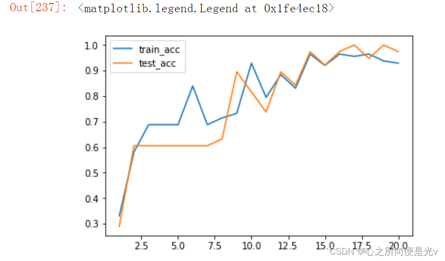


 1万+
1万+


 被折叠的 条评论
为什么被折叠?
被折叠的 条评论
为什么被折叠?
 到【灌水乐园】发言


