


 本文介绍“K邻居算法进行鸢尾花分类”项目,以K最近邻算法对鸢尾花数据集分类。先进行数据预处理、分析与可视化,再用KNN算法训练模型并选最优K值,最后评估性能。探讨不同K值对分类准确性的影响,助初学者理解数据处理与模型评估。
注意:本文引用自专业人工智能社区Venus AI
更多AI知识请参考原站 ([www.aideeplearning.cn])
项目简介:K邻居算法进行鸢尾花分类
概述 “K邻居算法进行鸢尾花分类”项目是一个基于机器学习的应用,旨在使用K最近邻(K-Nearest Neighbors, KNN)算法对鸢尾花数据集进行分类。该项目展示了如何通过KNN算法准确地识别和分类不同种类的鸢尾花,包括山鸢尾、变色鸢尾和维吉尼亚鸢尾。
项目背景 鸢尾花数据集是机器学习领域中最著名的数据集之一,常用于入门级教学和算法验证。该数据集包含150个样本,每个样本包含4个特征:萼片长度、萼片宽度、花瓣长度和花瓣宽度。基于这些特征,样本被分为三个鸢尾花种类。
技术实现 项目使用KNN算法作为核心分类器。KNN是一种简单但强大的非参数化分类算法,通过查找测试数据在特征空间中的K个最近邻居来预测分类。选择适当的K值对模型性能至关重要,因此项目中将探讨不同K值对分类准确性的影响。
项目结构
- 数据预处理:加载鸢尾花数据集,执行必要的清洗和归一化,进行数据分析和可视化。
- 模型训练:使用KNN算法训练模型,并通过交叉验证选择最优的K值。
- 性能评估:评估模型在测试数据集上的准确性。
- 结果分析:分析和解释KNN模型的结果,包括错误分类的观察和可能的改进方案。
应用意义 通过本项目,初学者不仅能学习到KNN算法的基本原理和实践应用,还能深入理解数据预处理、模型评估和超参数调优的重要性。此外,该项目还为理解和解决更复杂的分类问题奠定了基础。
数据分析
import numpy as np
import pandas as pd
import seaborn as sns
iris_data = pd.read_csv('Data/iris.csv')iris_info = iris_data.info()
iris_describe = iris_data.describe()
iris_head = iris_data.head()
print(iris_info)
print(iris_describe)
print(iris_head)<class 'pandas.core.frame.DataFrame'>
RangeIndex: 150 entries, 0 to 149
Data columns (total 6 columns):
# Column Non-Null Count Dtype
--- ------ -------------- -----
0 Id 150 non-null int64
1 SepalLengthCm 150 non-null float64
2 SepalWidthCm 150 non-null float64
3 PetalLengthCm 150 non-null float64
4 PetalWidthCm 150 non-null float64
5 Species 150 non-null object
dtypes: float64(4), int64(1), object(1)
memory usage: 7.2+ KB
None
Id SepalLengthCm SepalWidthCm PetalLengthCm PetalWidthCm
count 150.000000 150.000000 150.000000 150.000000 150.000000
mean 75.500000 5.843333 3.054000 3.758667 1.198667
std 43.445368 0.828066 0.433594 1.764420 0.763161
min 1.000000 4.300000 2.000000 1.000000 0.100000
25% 38.250000 5.100000 2.800000 1.600000 0.300000
50% 75.500000 5.800000 3.000000 4.350000 1.300000
75% 112.750000 6.400000 3.300000 5.100000 1.800000
max 150.000000 7.900000 4.400000 6.900000 2.500000
Id SepalLengthCm SepalWidthCm PetalLengthCm PetalWidthCm Species
0 1 5.1 3.5 1.4 0.2 Iris-setosa
1 2 4.9 3.0 1.4 0.2 Iris-setosa
2 3 4.7 3.2 1.3 0.2 Iris-setosa
3 4 4.6 3.1 1.5 0.2 Iris-setosa
4 5 5.0 3.6 1.4 0.2 Iris-setosa# 每个不同物种的描述性统计。
# 检查 3 个物种的平均花瓣长度
for t in iris_data['PetalLengthCm'].unique():
print(t)
print(iris_data[iris_data['PetalLengthCm'] == t].mean(numeric_only=True))1.4
Id 21.833333
SepalLengthCm 4.916667
SepalWidthCm 3.333333
PetalLengthCm 1.400000
PetalWidthCm 0.216667
dtype: float64
1.3
Id 31.714286
SepalLengthCm 4.842857
SepalWidthCm 3.228571
PetalLengthCm 1.300000
PetalWidthCm 0.257143
dtype: float64
1.5
Id 24.714286
SepalLengthCm 5.128571
SepalWidthCm 3.535714
PetalLengthCm 1.500000
PetalWidthCm 0.221429
dtype: float64
1.7
Id 17.50
SepalLengthCm 5.40
SepalWidthCm 3.60
PetalLengthCm 1.70
PetalWidthCm 0.35
dtype: float64
1.6
Id 31.000000
SepalLengthCm 4.914286
SepalWidthCm 3.342857
PetalLengthCm 1.600000
PetalWidthCm 0.285714
dtype: float64
1.1
Id 14.0
SepalLengthCm 4.3
SepalWidthCm 3.0
PetalLengthCm 1.1
PetalWidthCm 0.1
dtype: float64
1.2
Id 25.5
SepalLengthCm 5.4
SepalWidthCm 3.6
PetalLengthCm 1.2
PetalWidthCm 0.2
dtype: float64
1.0
Id 23.0
SepalLengthCm 4.6
SepalWidthCm 3.6
PetalLengthCm 1.0
PetalWidthCm 0.2
dtype: float64
1.9
Id 35.00
SepalLengthCm 4.95
SepalWidthCm 3.60
PetalLengthCm 1.90
PetalWidthCm 0.30
dtype: float64
4.7
Id 66.60
SepalLengthCm 6.44
SepalWidthCm 3.06
PetalLengthCm 4.70
PetalWidthCm 1.42
dtype: float64
4.5
Id 75.1250
SepalLengthCm 5.7750
SepalWidthCm 2.8750
PetalLengthCm 4.5000
PetalWidthCm 1.5125
dtype: float64
4.9
Id 100.00
SepalLengthCm 6.24
SepalWidthCm 2.82
PetalLengthCm 4.90
PetalWidthCm 1.72
dtype: float64
4.0
Id 74.40
SepalLengthCm 5.78
SepalWidthCm 2.48
PetalLengthCm 4.00
PetalWidthCm 1.22
dtype: float64
4.6
Id 68.666667
SepalLengthCm 6.400000
SepalWidthCm 2.900000
PetalLengthCm 4.600000
PetalWidthCm 1.400000
dtype: float64
3.3
Id 76.00
SepalLengthCm 4.95
SepalWidthCm 2.35
PetalLengthCm 3.30
PetalWidthCm 1.00
dtype: float64
3.9
Id 71.000000
SepalLengthCm 5.533333
SepalWidthCm 2.633333
PetalLengthCm 3.900000
PetalWidthCm 1.233333
dtype: float64
3.5
Id 70.50
SepalLengthCm 5.35
SepalWidthCm 2.30
PetalLengthCm 3.50
PetalWidthCm 1.00
dtype: float64
4.2
Id 87.500
SepalLengthCm 5.725
SepalWidthCm 2.900
PetalLengthCm 4.200
PetalWidthCm 1.325
dtype: float64
3.6
Id 65.0
SepalLengthCm 5.6
SepalWidthCm 2.9
PetalLengthCm 3.6
PetalWidthCm 1.3
dtype: float64
4.4
Id 80.250
SepalLengthCm 6.275
SepalWidthCm 2.750
PetalLengthCm 4.400
PetalWidthCm 1.325
dtype: float64
4.1
Id 85.666667
SepalLengthCm 5.700000
SepalWidthCm 2.833333
PetalLengthCm 4.100000
PetalWidthCm 1.200000
dtype: float64
4.8
Id 103.500
SepalLengthCm 6.225
SepalWidthCm 2.950
PetalLengthCm 4.800
PetalWidthCm 1.700
dtype: float64
4.3
Id 86.5
SepalLengthCm 6.3
SepalWidthCm 2.9
PetalLengthCm 4.3
PetalWidthCm 1.3
dtype: float64
5.0
Id 114.750
SepalLengthCm 6.175
SepalWidthCm 2.550
PetalLengthCm 5.000
PetalWidthCm 1.775
dtype: float64
3.8
Id 81.0
SepalLengthCm 5.5
SepalWidthCm 2.4
PetalLengthCm 3.8
PetalWidthCm 1.1
dtype: float64
3.7
Id 82.0
SepalLengthCm 5.5
SepalWidthCm 2.4
PetalLengthCm 3.7
PetalWidthCm 1.0
dtype: float64
5.1
Id 122.625
SepalLengthCm 6.125
SepalWidthCm 2.875
PetalLengthCm 5.100
PetalWidthCm 1.925
dtype: float64
3.0
Id 99.0
SepalLengthCm 5.1
SepalWidthCm 2.5
PetalLengthCm 3.0
PetalWidthCm 1.1
dtype: float64
6.0
Id 113.50
SepalLengthCm 6.75
SepalWidthCm 3.25
PetalLengthCm 6.00
PetalWidthCm 2.15
dtype: float64
5.9
Id 123.50
SepalLengthCm 6.95
SepalWidthCm 3.10
PetalLengthCm 5.90
PetalWidthCm 2.20
dtype: float64
5.6
Id 129.833333
SepalLengthCm 6.366667
SepalWidthCm 2.933333
PetalLengthCm 5.600000
PetalWidthCm 2.050000
dtype: float64
5.8
Id 114.666667
SepalLengthCm 6.800000
SepalWidthCm 2.833333
PetalLengthCm 5.800000
PetalWidthCm 1.866667
dtype: float64
6.6
Id 106.0
SepalLengthCm 7.6
SepalWidthCm 3.0
PetalLengthCm 6.6
PetalWidthCm 2.1
dtype: float64
6.3
Id 108.0
SepalLengthCm 7.3
SepalWidthCm 2.9
PetalLengthCm 6.3
PetalWidthCm 1.8
dtype: float64
6.1
Id 125.666667
SepalLengthCm 7.433333
SepalWidthCm 3.133333
PetalLengthCm 6.100000
PetalWidthCm 2.233333
dtype: float64
5.3
Id 114.00
SepalLengthCm 6.40
SepalWidthCm 2.95
PetalLengthCm 5.30
PetalWidthCm 2.10
dtype: float64
5.5
Id 122.666667
SepalLengthCm 6.566667
SepalWidthCm 3.033333
PetalLengthCm 5.500000
PetalWidthCm 1.900000
dtype: float64
6.7
Id 120.5
SepalLengthCm 7.7
SepalWidthCm 3.3
PetalLengthCm 6.7
PetalWidthCm 2.1
dtype: float64
6.9
Id 119.0
SepalLengthCm 7.7
SepalWidthCm 2.6
PetalLengthCm 6.9
PetalWidthCm 2.3
dtype: float64
5.7
Id 130.333333
SepalLengthCm 6.766667
SepalWidthCm 3.266667
PetalLengthCm 5.700000
PetalWidthCm 2.300000
dtype: float64
6.4
Id 132.0
SepalLengthCm 7.9
SepalWidthCm 3.8
PetalLengthCm 6.4
PetalWidthCm 2.0
dtype: float64
5.4
Id 144.50
SepalLengthCm 6.55
SepalWidthCm 3.25
PetalLengthCm 5.40
PetalWidthCm 2.20
dtype: float64
5.2
Id 147.00
SepalLengthCm 6.60
SepalWidthCm 3.00
PetalLengthCm 5.20
PetalWidthCm 2.15
dtype: float64可视化数据
iris_data.head()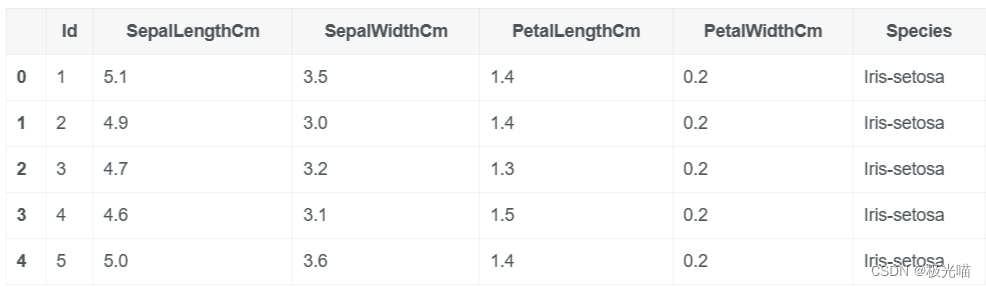
Boxplot
sns.boxplot(x='Species',
                y='PetalLengthCm',
data=iris_data) 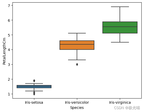
我们可以看到sentosa的花瓣长度与其他两个花瓣分开。 然而,“Versicolor”和“Virgina”之间的花瓣长度是重叠的。 因此,我们可能无法单独使用“PetalLengthCm”特征来区分物种。
Violin Plot
sns.violinplot(x = 'Species',
                      y = 'PetalWidthCm',
data = iris_data) 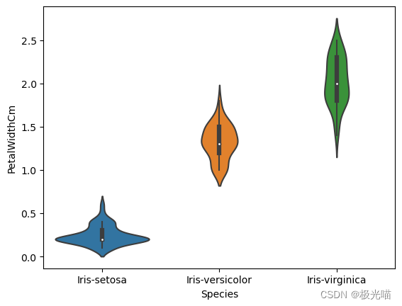
从上表可以看出,“setosa”的“PetalWidthCM”大部分约为 0.25 厘米,“versicolor”的花瓣宽度约为 1.3 至 1.5 厘米。 对于“virginica”来说,除了 1.9 左右之外,它实际上并没有显着的分布。 正如前面提到的,PetalWidth 的 versicolor 和 virginica 之间也有很多重叠。
Pair Plot
- 查看数据特征如何相互交互的快速方法
我们发现,要识别“sentosa”,我们可以纯粹使用“PetalLeghtCM”。 但为了区分“versicolor”和“virginica”,我们需要更多信息。
sns.pairplot(data = iris_data.drop('Id',axis =1),
hue='Species') 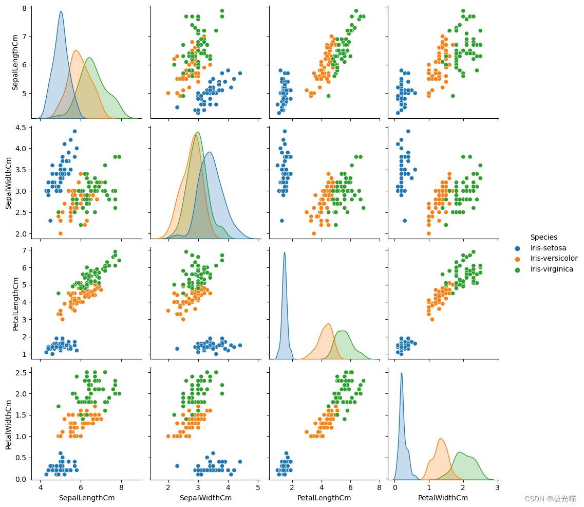
根据上图,我们可以看到“PetalLengthCm”和“PetalWidthCm”对图是最清晰的区分不同物种的方式。
训练模型
import numpy as np
import pandas as pd

from sklearn.neighbors import KNeighborsClassifier

from mlxtend.plotting import plot_decision_regions
import matplotlib.pyplot as plt
%matplotlib inline
iris_data = pd.read_csv('Data/iris.csv')iris_data.head()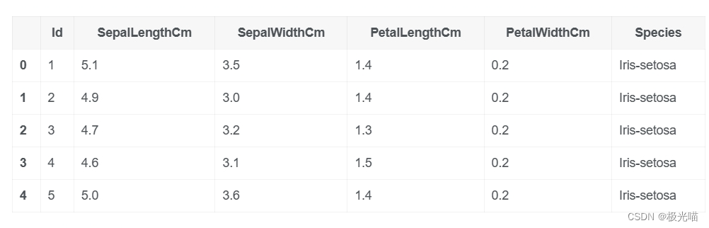
设置特征和标签
# features
X = iris_data[['PetalLengthCm','PetalWidthCm']]
X.head()
# labels
flower_type = {
    'Iris-setosa': 1,
    'Iris-versicolor': 2,
    'Iris-virginica': 3,
}
# 将物种映射到数值
y = iris_data['Species'].map(flower_type)
y.head()0 1
1 1
2 1
3 1
4 1
Name: Species, dtype: int64训练KNN模型 (6 neighbors)
knn = KNeighborsClassifier(n_neighbors=6)

knn.fit(X, y)
绘制决策边界
plot_decision_regions(np.array(X), np.array(y), clf=knn, legend=2)

plt.xlabel('PetalLengthCm')
plt.ylabel('PetalWidthCm')
plt.title('knn on Iris with 2 features')
plt.show() 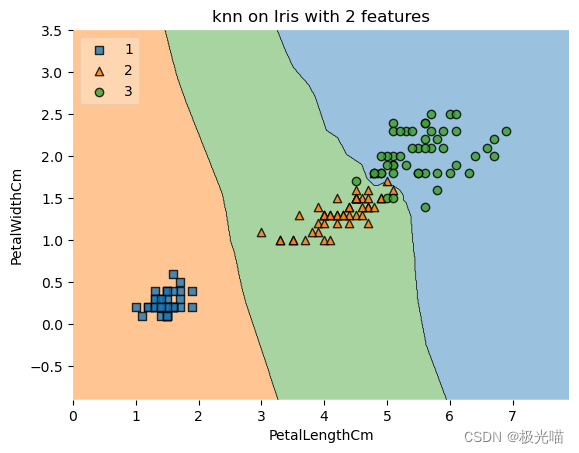
训练KNN模型 (20 neighbors)
knn = KNeighborsClassifier(n_neighbors = 20)
knn.fit(X, y)
plot_decision_regions(np.array(X), np.array(y), clf=knn, legend=2)
plt.xlabel('PetalLengthCm')
plt.ylabel('PetalWidthCm')
plt.title('knn on Iris with 2 features')
plt.show() 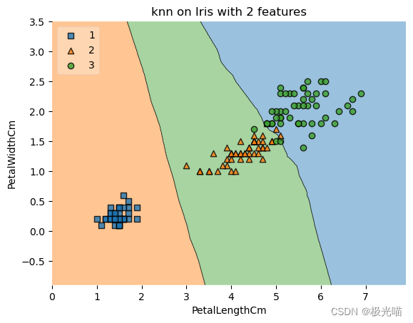
评估模型
import pandas as pd
from sklearn.model_selection import train_test_split
from sklearn.neighbors import KNeighborsClassifier
from sklearn.metrics import accuracy_score, precision_score, recall_score

iris_data = pd.read_csv('Data/iris.csv')
iris_data.head()

# features
features = iris_data[['PetalLengthCm','SepalLengthCm','PetalWidthCm','SepalWidthCm']]
# labels
flowers = {
    'Iris-setosa':1,
    'Iris-versicolor':2,
    'Iris-virginica':3
}

labels = iris_data['Species'].map(flowers)

X_train, X_test, y_train, y_test = train_test_split(features, labels, test_size=0.8, random_state=64)

knn = KNeighborsClassifier(n_neighbors=3)
knn.fit(X_train, y_train)

# check with test dataset
predict = knn.predict(X_test)

# check the predicted results
print(accuracy_score(predict, y_test))
print(precision_score(predict, y_test, average='weighted'))
print(recall_score(predict, y_test, average='weighted'))

# check the predicted results
print(accuracy_score(predict, y_test))
print(precision_score(predict, y_test, average=None))
print(recall_score(predict, y_test, average=None))


 5422
5422

 被折叠的 条评论
为什么被折叠?
被折叠的 条评论
为什么被折叠?
 到【灌水乐园】发言


