使用Sklearn进行精确率-召回率曲线的绘制

使用Sklearn进行精确率-召回率曲线的绘制

• 精确率：模型判定的正例中真正正例所占的比重
• 召回率：总正例中被模型判定为正例的比重

#coding=utf-8
"""
#演示目的：利用鸢尾花数据集画出P-R曲线
"""
print(__doc__)

#演示目的：利用鸢尾花数据集画出P-R曲线

import matplotlib.pyplot as plt
import numpy as np
from sklearn import svm, datasets
from sklearn.metrics import precision_recall_curve
from sklearn.metrics import average_precision_score
from sklearn.preprocessing import label_binarize
from sklearn.multiclass import OneVsRestClassifier
#from sklearn.cross_validation import train_test_split  #适用于anaconda 3.6及以前版本
from sklearn.model_selection import train_test_split#适用于anaconda 3.7

#以iris数据为例，画出P-R曲线
iris = datasets.load_iris()
X = iris.data
y = iris.target
print(y)
# 标签二值化,将三个类转为001, 010, 100的格式.因为这是个多类分类问题，后面将要采用
#OneVsRestClassifier策略转为二类分类问题
y = label_binarize(y, classes=[0, 1, 2])
n_classes = y.shape[1]
print(y.shape)
print (y)

# 增加了800维的 噪声特征
random_state = np.random.RandomState(0)
n_samples, n_features = X.shape
# print(X.shape)  (150, 4)
X = np.c_[X, random_state.randn(n_samples, 200 * n_features)]
# print(X.shape)  (150, 804)
# Split into training and test
X_train, X_test, y_train, y_test = train_test_split(X, y, test_size=.5, random_state=random_state) #随机数，填0或不填，每次都会不一样

# Run classifier probability : boolean, optional (default=False)Whether to enable probability estimates. This must be enabled prior to calling fit, and will slow down that method.
classifier = OneVsRestClassifier(svm.SVC(kernel='linear', probability=True, random_state=random_state))
y_score = classifier.fit(X_train, y_train).decision_function(X_test)

[0 0 0 0 0 0 0 0 0 0 0 0 0 0 0 0 0 0 0 0 0 0 0 0 0 0 0 0 0 0 0 0 0 0 0 0 0
 0 0 0 0 0 0 0 0 0 0 0 0 0 1 1 1 1 1 1 1 1 1 1 1 1 1 1 1 1 1 1 1 1 1 1 1 1
 1 1 1 1 1 1 1 1 1 1 1 1 1 1 1 1 1 1 1 1 1 1 1 1 1 1 2 2 2 2 2 2 2 2 2 2 2
 2 2 2 2 2 2 2 2 2 2 2 2 2 2 2 2 2 2 2 2 2 2 2 2 2 2 2 2 2 2 2 2 2 2 2 2 2
 2 2]
(150, 3)
[[1 0 0]
 [1 0 0]
 [1 0 0]
 [1 0 0]
 [1 0 0]
 [1 0 0]
 [1 0 0]
 [1 0 0]
 [1 0 0]
 [1 0 0]
 [1 0 0]
 [1 0 0]
 [1 0 0]
 [1 0 0]
 [1 0 0]
 [1 0 0]
 [1 0 0]
 [1 0 0]
 [1 0 0]
 [1 0 0]
 [1 0 0]
 [1 0 0]
 [1 0 0]
 [1 0 0]
 [1 0 0]
 [1 0 0]
 [1 0 0]
 [1 0 0]
 [1 0 0]
 [1 0 0]
 [1 0 0]
 [1 0 0]
 [1 0 0]
 [1 0 0]
 [1 0 0]
 [1 0 0]
 [1 0 0]
 [1 0 0]
 [1 0 0]
 [1 0 0]
 [1 0 0]
 [1 0 0]
 [1 0 0]
 [1 0 0]
 [1 0 0]
 [1 0 0]
 [1 0 0]
 [1 0 0]
 [1 0 0]
 [1 0 0]
 [0 1 0]
 [0 1 0]
 [0 1 0]
 [0 1 0]
 [0 1 0]
 [0 1 0]
 [0 1 0]
 [0 1 0]
 [0 1 0]
 [0 1 0]
 [0 1 0]
 [0 1 0]
 [0 1 0]
 [0 1 0]
 [0 1 0]
 [0 1 0]
 [0 1 0]
 [0 1 0]
 [0 1 0]
 [0 1 0]
 [0 1 0]
 [0 1 0]
 [0 1 0]
 [0 1 0]
 [0 1 0]
 [0 1 0]
 [0 1 0]
 [0 1 0]
 [0 1 0]
 [0 1 0]
 [0 1 0]
 [0 1 0]
 [0 1 0]
 [0 1 0]
 [0 1 0]
 [0 1 0]
 [0 1 0]
 [0 1 0]
 [0 1 0]
 [0 1 0]
 [0 1 0]
 [0 1 0]
 [0 1 0]
 [0 1 0]
 [0 1 0]
 [0 1 0]
 [0 1 0]
 [0 1 0]
 [0 1 0]
 [0 1 0]
 [0 0 1]
 [0 0 1]
 [0 0 1]
 [0 0 1]
 [0 0 1]
 [0 0 1]
 [0 0 1]
 [0 0 1]
 [0 0 1]
 [0 0 1]
 [0 0 1]
 [0 0 1]
 [0 0 1]
 [0 0 1]
 [0 0 1]
 [0 0 1]
 [0 0 1]
 [0 0 1]
 [0 0 1]
 [0 0 1]
 [0 0 1]
 [0 0 1]
 [0 0 1]
 [0 0 1]
 [0 0 1]
 [0 0 1]
 [0 0 1]
 [0 0 1]
 [0 0 1]
 [0 0 1]
 [0 0 1]
 [0 0 1]
 [0 0 1]
 [0 0 1]
 [0 0 1]
 [0 0 1]
 [0 0 1]
 [0 0 1]
 [0 0 1]
 [0 0 1]
 [0 0 1]
 [0 0 1]
 [0 0 1]
 [0 0 1]
 [0 0 1]
 [0 0 1]
 [0 0 1]
 [0 0 1]
 [0 0 1]
 [0 0 1]]

# Compute Precision-Recall and plot curve  
#下面的下划线是返回的阈值。作为一个名称：此时“_”作为临时性的名称使用。
#表示分配了一个特定的名称，但是并不会在后面再次用到该名称。
precision = dict()
recall = dict()
average_precision = dict()

for i in range(n_classes):
    precision[i], recall[i], _ = precision_recall_curve(y_test[:, i],  y_score[:, i]) #The last precision and recall values are 1. and 0. respectively and do not have a corresponding threshold. This ensures that the graph starts on the x axis.
    average_precision[i] = average_precision_score(y_test[:, i], y_score[:, i])#切片，第i个类的分类结果性能

# Compute micro-average curve and area. ravel()将多维数组降为一维
precision["micro"], recall["micro"], _ = precision_recall_curve(y_test.ravel(),  y_score.ravel())
average_precision["micro"] = average_precision_score(y_test, y_score, average="micro") #This score corresponds to the area under the precision-recall curve.

# Plot Precision-Recall curve for each class
plt.clf()#clf 函数用于清除当前图像窗口
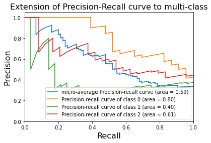
plt.plot(recall["micro"], precision["micro"],
         label='micro-average Precision-recall curve (area = {0:0.2f})'.format(average_precision["micro"]))
for i in range(n_classes):
    plt.plot(recall[i], precision[i],
             label='Precision-recall curve of class {0} (area = {1:0.2f})'.format(i, average_precision[i]))

plt.xlim([0.0, 1.0])
plt.ylim([0.0, 1.05]) #xlim、ylim：分别设置X、Y轴的显示范围。
plt.xlabel('Recall', fontsize=16)
plt.ylabel('Precision',fontsize=16)
plt.title('Extension of Precision-Recall curve to multi-class',fontsize=16)
plt.legend(loc="lower right")#legend 是用于设置图例的函数
plt.show()