机器学习实战（六）：Decision Trees

最新推荐文章于 2022-11-15 14:20:36 发布

一城山河

最新推荐文章于 2022-11-15 14:20:36 发布

阅读量341

点赞数

分类专栏：机器学习文章标签：决策树机器学习深度学习 python

本文链接：https://blog.csdn.net/qq_40594395/article/details/111035900

版权

机器学习专栏收录该内容

14 篇文章 3 订阅

订阅专栏

决策树也像SVM一样能实现分类与回归（甚至多输出），能拟合复杂数据集。
本章将训练、可视化、预测决策树，介绍Scikit-Learn的CART算法，介绍正则化决策树并应用于回归，介绍决策树的部分限制。

Training and Visualizing a Decision Tree

构建决策树，了解其如何预测（load_iris）：

from sklearn.datasets import load_iris
from sklearn.tree import DecisionTreeClassifier

iris = load_iris()
X = iris.data[:, 2:] # petal length and width
y = iris.target

tree_clf = DecisionTreeClassifier(max_depth=2, random_state=42)
tree_clf.fit(X, y)

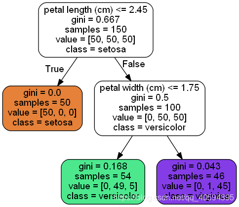
可视化决策树：用export——graphviz()输出iris_tree.dot文件：


from sklearn.tree import export_graphviz

export_graphviz(
        tree_clf,
        out_file=image_path("iris_tree.dot"),
        feature_names=iris.feature_names[2:],
        class_names=iris.target_names,
        rounded=True,
        filled=True
    )

用graphviz包（需要事先安装）dot命令转换格式：dot -Tpng iris_tree.dot -o iris_tree.png
在这里插入图片描述

Making Predictions

看图的话预测过程就比较清晰了，从根节点开始，先看花瓣长度是否<=2.45cm,然后跟着图的思路一步步到叶节点。

决策树的特质之一：需要数据准备非常少，完全不需要特征集中或缩放。

解释一下图中几个属性：

samples：统计与应用的训练实例数量
value：该节点上每个类别训练实例数量
gini：不纯度（纯为0）

gini不纯度计算公式：pik:第i个节点上，类别为k的训练实例占比
在这里插入图片描述

Scikit-Learn使用CART算法仅生成二叉树；ID3生成决策树

看一下决策边界：

from matplotlib.colors import ListedColormap

def plot_decision_boundary(clf, X, y, axes=[0, 7.5, 0, 3], iris=True, legend=False, plot_training=True):
    x1s = np.linspace(axes[0], axes[1], 100)
    x2s = np.linspace(axes[2], axes[3], 100)
    x1, x2 = np.meshgrid(x1s, x2s)
    X_new = np.c_[x1.ravel(), x2.ravel()]
    y_pred = clf.predict(X_new).reshape(x1.shape)
    custom_cmap = ListedColormap(['#fafab0','#9898ff','#a0faa0'])
    plt.contourf(x1, x2, y_pred, alpha=0.3, cmap=custom_cmap)
    if not iris:
        custom_cmap2 = ListedColormap(['#7d7d58','#4c4c7f','#507d50'])
        plt.contour(x1, x2, y_pred, cmap=custom_cmap2, alpha=0.8)
    if plot_training:
        plt.plot(X[:, 0][y==0], X[:, 1][y==0], "yo", label="Iris-Setosa")
        plt.plot(X[:, 0][y==1], X[:, 1][y==1], "bs", label="Iris-Versicolor")
        plt.plot(X[:, 0][y==2], X[:, 1][y==2], "g^", label="Iris-Virginica")
        plt.axis(axes)
    if iris:
        plt.xlabel("Petal length", fontsize=14)
        plt.ylabel("Petal width", fontsize=14)
    else:
        plt.xlabel(r"$x_1$", fontsize=18)
        plt.ylabel(r"$x_2$", fontsize=18, rotation=0)
    if legend:
        plt.legend(loc="lower right", fontsize=14)

plt.figure(figsize=(8, 4))
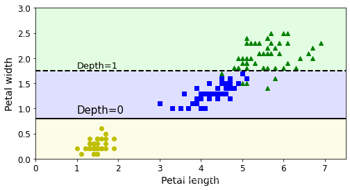
plot_decision_boundary(tree_clf, X, y)
plt.plot([2.45, 2.45], [0, 3], "k-", linewidth=2)
plt.plot([2.45, 7.5], [1.75, 1.75], "k--", linewidth=2)
plt.plot([4.95, 4.95], [0, 1.75], "k:", linewidth=2)
plt.plot([4.85, 4.85], [1.75, 3], "k:", linewidth=2)
plt.text(1.40, 1.0, "Depth=0", fontsize=15)
plt.text(3.2, 1.80, "Depth=1", fontsize=13)
plt.text(4.05, 0.5, "(Depth=2)", fontsize=11)

在这里插入图片描述
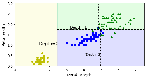
如图所示，2.45决策边界（深度为1），1.75决策边界（深度为2），若max_depth=3则dot-line将成为第三个决策边界。

决策树是白盒模型（直观容易解释），随机森林神经网络是黑盒模型（难以解释为什么这样预测）

Estimating Class Probabilities（估算类别概率）：

决策树估算类别概率：找出类别k叶子节点：返回k实例占比：tree_clf.predict_proba([[5, 1.5]])
输出array([[0. , 0.90740741, 0.09259259]])，输出tree_clf.predict_proba([[6, 1.5]])结果相同。

The CART Training Algorithm

Scikit-Learn使用的是分类与回归树（Classification And Regression Tree——CART）训练决策树（生长树)：首先使用特征k和阈值tk训练成两个子集，k，tk的选择：最纯子集（加权）的k，tk，算法函数：
在这里插入图片描述

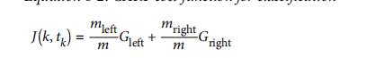
Gleft/right：衡量左右子集的不纯度
mleft/right：左/右子集实例数量

分裂子集直至抵达max_depth,或再也找不到能够降低不纯度的分裂，附加停止条件（min_samples_split, min_samples_leaf, min_weight_fraction_leaf, and max_leaf_nodes）

CART是贪婪算法：从顶层开始搜索最优分裂，每层重复，但不保证是最优解。而且寻找最优树是NP完全问题（NP：能在多项式时间内验证正确，L 是NP-Hard，任何一个NP问题都可以在多项式时间内被规划成L问题，NP完全：既是NP又是NP-Hard），所以必须接受CART是一个相对不错解。

Computational Complexity

预测是从根到叶：O（log2（m））个节点，与特征数量无关。
但训练是要在所有样本上比较所有特征（除非设置max_features）,导致复杂度O（n*m log（m））小型数据集可以通过设置 presort = "true"来解决，大型就得放缓速度。

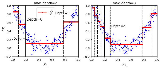
Gini Impurity or Entropy?（Gini不纯度还是信息熵？）

默认是gini 不纯度来测量，可以通过 criterion = "entropy"来选择信息熵做不纯度测量，计算：
在这里插入图片描述

Regularization Hyperparameters（正则化超参数）

决策树很少对训练数据做假设（线性模型相反，假设线性）。非参数模型：如果不限制，树结构将随训练集变化，便过拟合。（训练前没有确定参数数量，即过度拟合）

所以需要降低决策树自由度——正则化。正则化超参数取决于所用模型，例如max_depth，减小max_depth可使模型正则化，降低过度拟合风险。
其他参数：

min_samples_split：分裂前必须有的最小样本数量
min_samples_leaf：叶子节点必须有的最小样本数量
min_weight_fraction_leaf：叶子节点必须有的最小样本占比
max_leaf_nodes：最大叶节点数量
max_features：分裂每个节点评估的最大特征数量

还有一种正则化：先不加约束训练，再对不必要节点删除：若一个节点子节点全为叶节点，则没必要（除非有利于提纯）；标准统计测试，如 χ2测试（估算提纯出于偶然——虚假设）概率，高于阈值，子节点可删。直至所有不必要节点都被删掉。

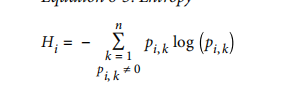
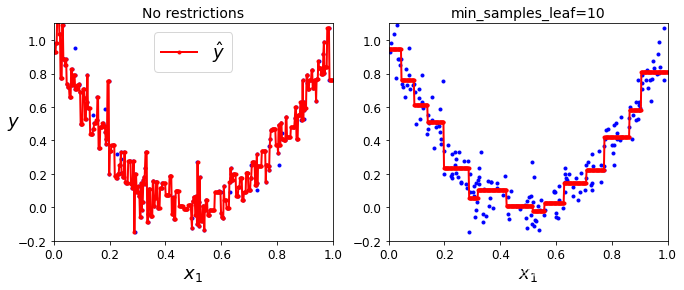
from sklearn.datasets import make_moons
Xm, ym = make_moons(n_samples=100, noise=0.25, random_state=53)

deep_tree_clf1 = DecisionTreeClassifier(random_state=42)
deep_tree_clf2 = DecisionTreeClassifier(min_samples_leaf=4, random_state=42)
deep_tree_clf1.fit(Xm, ym)
deep_tree_clf2.fit(Xm, ym)

plt.figure(figsize=(11, 4))
plt.subplot(121)
plot_decision_boundary(deep_tree_clf1, Xm, ym, axes=[-1.5, 2.5, -1, 1.5], iris=False)
plt.title("No restrictions", fontsize=16)
plt.subplot(122)
plot_decision_boundary(deep_tree_clf2, Xm, ym, axes=[-1.5, 2.5, -1, 1.5], iris=False)
plt.title("min_samples_leaf = {}".format(deep_tree_clf2.min_samples_leaf), fontsize=14)

在这里插入图片描述
右图应用min_samples_leaf =4，明显泛化更好，左图过拟合。

Regression

决策树回归：例：Scikit-Learn的DecisionTreeRegressor（max_depth= 2）加噪声的二次数据集训练：
构建数据集：

# Quadratic training set + noise
np.random.seed(42)
m = 200
X = np.random.rand(m, 1)
y = 4 * (X - 0.5) ** 2
y = y + np.random.randn(m, 1) / 10

训练模型：

from sklearn.tree import DecisionTreeRegressor
tree_reg = DecisionTreeRegressor(max_depth=2, random_state=42)
tree_reg.fit(X, y)

在这里插入图片描述
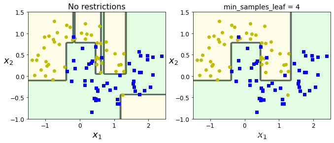
结果树如图，跟分类树相似，差别是从预测一个结果转变为预测一个值。例：x1 = 0.6 到value = 0.1106的叶节点，预测结果为此节点110个实例平均值。测出MSE = 0.0151.

from sklearn.tree import DecisionTreeRegressor

tree_reg1 = DecisionTreeRegressor(random_state=42, max_depth=2)
tree_reg2 = DecisionTreeRegressor(random_state=42, max_depth=3)
tree_reg1.fit(X, y)
tree_reg2.fit(X, y)

def plot_regression_predictions(tree_reg, X, y, axes=[0, 1, -0.2, 1], ylabel="$y$"):
    x1 = np.linspace(axes[0], axes[1], 500).reshape(-1, 1)
    y_pred = tree_reg.predict(x1)
    plt.axis(axes)
    plt.xlabel("$x_1$", fontsize=18)
    if ylabel:
        plt.ylabel(ylabel, fontsize=18, rotation=0)
    plt.plot(X, y, "b.")
    plt.plot(x1, y_pred, "r.-", linewidth=2, label=r"$\hat{y}$")

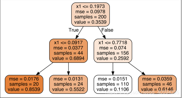
plt.figure(figsize=(11, 4))
plt.subplot(121)
plot_regression_predictions(tree_reg1, X, y)
for split, style in ((0.1973, "k-"), (0.0917, "k--"), (0.7718, "k--")):
    plt.plot([split, split], [-0.2, 1], style, linewidth=2)
plt.text(0.21, 0.65, "Depth=0", fontsize=15)
plt.text(0.01, 0.2, "Depth=1", fontsize=13)
plt.text(0.65, 0.8, "Depth=1", fontsize=13)
plt.legend(loc="upper center", fontsize=18)
plt.title("max_depth=2", fontsize=14)

plt.subplot(122)
plot_regression_predictions(tree_reg2, X, y, ylabel=None)
for split, style in ((0.1973, "k-"), (0.0917, "k--"), (0.7718, "k--")):
    plt.plot([split, split], [-0.2, 1], style, linewidth=2)
for split in (0.0458, 0.1298, 0.2873, 0.9040):
    plt.plot([split, split], [-0.2, 1], "k:", linewidth=1)
plt.text(0.3, 0.5, "Depth=2", fontsize=13)
plt.title("max_depth=3", fontsize=14)

在这里插入图片描述
若设max_depth = 2，则是右图，预测值为该区域实例目标平均值，算法分裂实质就是更接近预测值。

CART原理也是这样，但它分裂训练集方式是最小化MSE，而不是最小化不纯度，下图为最小化不纯度成本函数：
在这里插入图片描述
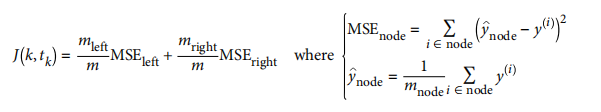
无论是回归还是分类，都很容易过拟合。

如图所示，左图过拟合，右图设置max_samples_leaf = 10后后很多。
代码：


tree_reg1 = DecisionTreeRegressor(random_state=42)
tree_reg2 = DecisionTreeRegressor(random_state=42, min_samples_leaf=10)
tree_reg1.fit(X, y)
tree_reg2.fit(X, y)

x1 = np.linspace(0, 1, 500).reshape(-1, 1)
y_pred1 = tree_reg1.predict(x1)
y_pred2 = tree_reg2.predict(x1)

plt.figure(figsize=(11, 4))

plt.subplot(121)
plt.plot(X, y, "b.")
plt.plot(x1, y_pred1, "r.-", linewidth=2, label=r"$\hat{y}$")
plt.axis([0, 1, -0.2, 1.1])
plt.xlabel("$x_1$", fontsize=18)
plt.ylabel("$y$", fontsize=18, rotation=0)
plt.legend(loc="upper center", fontsize=18)
plt.title("No restrictions", fontsize=14)

plt.subplot(122)
plt.plot(X, y, "b.")
plt.plot(x1, y_pred2, "r.-", linewidth=2, label=r"$\hat{y}$")
plt.axis([0, 1, -0.2, 1.1])
plt.xlabel("$x_1$", fontsize=18)
plt.title("min_samples_leaf={}".format(tree_reg2.min_samples_leaf), fontsize=14)

Instability（不稳定性）

决策树容易解释理解，功能也很强大，但也有限制：对决策边界非常敏感，所以如果训练集旋转，则预测可能发生很大改变，改变这种现象就得使用PCA。
在这里插入图片描述

其实说敏感，敏感的是训练数据小变化，如果把最卷的V花删了，则重新训练
在这里插入图片描述
与以前训练（下图）差距很大。。
因为Scikit-Learn算法随机，所以相同训练数据，模型都可能完全不同（除非设置random_state）
下账将看到随机森林对多个树预测平均，限制不稳定性。

一城山河

关注

0
点赞
踩
1

收藏

觉得还不错? 一键收藏
0
评论
机器学习实战（六）：Decision Trees

决策树也像SVM一样能实现分类与回归（甚至多输出），能拟合复杂数据集。本章将训练、可视化、预测决策树，介绍Scikit-Learn的CART算法，介绍正则化决策树并应用于回归，介绍决策树的部分限制。Training and Visualizing a Decision Tree构建决策树，了解其如何预测（load_iris）：from sklearn.datasets import load_irisfrom sklearn.tree import DecisionTreeClassifier
复制链接

扫一扫