


目录
前言
最近有个需求,需要测试下 tensorRT 模型的性能,最近看了杜老师 tensorRT_Pro 这个 repo 中的方法,简单的实现了下,故此做个记录下方便下次查看。此次对 tensorRT 模型的测试主要包括 mAP 测试和速度测试,具体细节,大家自行查阅相关代码,这里只简单分享下博主在测试时实现的流程。
测试环境:NVIDIA RTX 3060,Ubuntu20.04,CUDA-11.6,cuDNN-8.4.0,tensorRT-8.4.1,OpenCV-4.6.0,protouf-3.11.4,pytorch-1.12.0
先说下测试大致的一个流程:
mAP 测试:模型训练 -> 导出 onnx -> 生成 FP32/FP16 模型 -> FP32/FP16/INT8 推理预测 -> 将结果保存为 JSON 文件 -> COCO Python API 测试 mAP
速度测试:模型训练 -> 导出 onnx -> 生成 FP32/FP16 模型 -> FP32/FP16/INT8 推理预测 -> warmup -> 循环推理计算平均推理时间
若有问题欢迎各位看官批评指正😀。OK,让我们开始吧!!!🚀🚀🚀
1. 模型训练
首先我们需要利用 pytorch 深度学习框架来训练两个模型
1.1 模型
博主这次选择测试了两个模型:YOLOv5m.pt 和 YOLOv6s.pt,直接选用 master 分支进行训练,测试代码均下载于 2023/7/22 日,下面是两个项目的地址:
1.2 数据集
博主没找到一个比较有意思的目标检测数据集,还是拿 VOC 来测试吧。
训练集:(VOC2007train + VOC2007val) * 80% = 4013
验证集:(VOC2007train + VOC2007val) * 20% = 998
测试集:无
关于VOC数据集的相关介绍和下载可参考 目标检测:PASCAL VOC 数据集简介
1.3 xml2yolo
拿到手的 VOC 数据集是 XML 格式的与 YOLO 格式要求的 txt 标签不符合,需要进行转换,转换代码如下:(from chatGPT)
import os
import cv2
import xml.etree.ElementTree as ET
import shutil
from multiprocessing import Pool, cpu_count
from tqdm import tqdm
import numpy as np
from functools import partial

def process_xml(xml_filename, img_path, xml_path, img_save_path, label_save_path, class_dict, ratio):
    # 解析 xml 文件
    xml_file_path = os.path.join(xml_path, xml_filename)
    tree = ET.parse(xml_file_path)
    root = tree.getroot()

    # 获取图像的宽度和高度
    img_filename = os.path.splitext(xml_filename)[0] + ".jpg"
    img = cv2.imread(os.path.join(img_path, img_filename))
    height, width = img.shape[:2]

    # 随机决定当前图像和标签是属于训练集还是验证集
    subset = "train" if np.random.random() < ratio else "val"

    # 打开对应的标签文件进行写入
    label_file = os.path.join(label_save_path, subset, os.path.splitext(xml_filename)[0] + ".txt")
    with open(label_file, "w") as file:
        for obj in root.iter('object'):
            # 获取类别名并转换为类别ID
            class_name = obj.find('name').text
            class_id = class_dict[class_name]

            # 获取并处理边界框的坐标
            xmlbox = obj.find('bndbox')
            x1 = float(xmlbox.find('xmin').text)
            y1 = float(xmlbox.find('ymin').text)
            x2 = float(xmlbox.find('xmax').text)
            y2 = float(xmlbox.find('ymax').text)

            # 计算中心点坐标和宽高,并归一化
            x_center = (x1 + x2) / 2 / width
            y_center = (y1 + y2) / 2 / height
            w = (x2 - x1) / width
            h = (y2 - y1) / height

            # 写入文件
            file.write(f"{class_id} {x_center} {y_center} {w} {h}\n")

    # 将图像文件复制到对应的训练集或验证集目录
    shutil.copy(os.path.join(img_path, img_filename), os.path.join(img_save_path, subset, img_filename))

def check_and_create_dir(path):
    # 检查并创建 train 和 val 目录
    for subset in ['train', 'val']:
        if not os.path.exists(os.path.join(path, subset)):
            os.makedirs(os.path.join(path, subset))

if __name__ == "__main__":
    # 1. 定义路径和类别字典,不要使用中文路径
    img_path = "D:\\Data\\PASCAL_VOC\\VOCdevkit\\VOC2007\\JPEGImages"
    xml_path = "D:\\Data\\PASCAL_VOC\\VOCdevkit\\VOC2007\\Annotations"
    img_save_path = "D:\\Data\\PASCAL_VOC\\dataset\\images"
    label_save_path = "D:\\Data\\PASCAL_VOC\\dataset\\labels"

    class_dict = {
    "aeroplane": 0,
    "bicycle": 1,
    "bird": 2,
    "boat": 3,
    "bottle": 4,
    "bus": 5,
    "car": 6,
    "cat": 7,
    "chair": 8,
    "cow": 9,
    "diningtable": 10,
    "dog": 11,
    "horse": 12,
    "motorbike": 13,
    "person": 14,
    "pottedplant": 15,
    "sheep": 16,
    "sofa": 17,
    "train": 18,
    "tvmonitor": 19
}

    train_val_ratio = 0.8  # 2. 定义训练集和验证集的比例

    # 检查并创建必要的目录
    check_and_create_dir(img_save_path)
    check_and_create_dir(label_save_path)

    # 获取 xml 文件列表
    xml_filenames = os.listdir(xml_path)

    # 创建进程池并执行
    with Pool(cpu_count()) as p:
        list(tqdm(p.imap(partial(process_xml, img_path=img_path, xml_path=xml_path, img_save_path=img_save_path, label_save_path=label_save_path,
                                 class_dict=class_dict, ratio=train_val_ratio), xml_filenames), total=len(xml_filenames)))
上述代码的功能是将 PASCAL VOC 格式的数据集(包括 JPEG 图像和 XML 格式的标注文件)转换成 YOLO 需要的数据格式。同时会将转换后的数据集按照 train_val_ratio 这个变量提供的比例随机划分为训练集和验证集,图像数据存储在 images/train 和 images/val 下面,标签文件存储在 labels/train labels/val 下面。
下面是这段代码的详细解释:(form chatGPT)
1. process_xml 函数:此函数处理单个 XML 文件,将其转换为 YOLO 格式的标签文件,并将对应的图像文件复制到正确的文件夹。它首先读取 XML 文件并解析其中的信息,包括图像尺寸、物体类别、物体的边界框坐标。然后,它根据一个随机数将数据分配给训练集或验证集。接着,它会创建一个新的 YOLO 格式的标签文件,并将物体的类别和归一化的边界框信息(中心点坐标和宽高)写入文件。最后,它会将原始的图像文件复制到对应的训练集或验证集的文件夹。
2. check_and_create_dir 函数:此函数检查并创建所需的目录。如果目录不存在,它会创建新的目录。
3. if __name__ == "__main__" 部分:这部分代码定义了文件和目录路径,类别字典,训练集和验证集的比例。然后,它调用 check_and_create_dir 函数来创建所需的目录。接着,它获取 XML 文件列表,创建一个进程池,并使用多进程的方式调用 process_xml 函数来处理所有的 XML 文件。
注意,这段代码使用了多进程来加速处理过程,因此它会尽可能利用所有可用的 CPU 核心。而 tqdm 库则用于显示处理进度。
这段代码假设你的数据集是 PASCAL VOC 格式的,也就是说你的标注文件是 XML 格式的,每个文件包含一个或多个 object 标签,每个 object 标签中包含一个 name 标签(表示类别名称)和一个 bndbox 标签(包含边界框的 xmin、ymin、xmax、ymax 坐标)。
你需要修改以下几项:
- img_path:存储着需要转换的 XML 标签文件对应的图像文件路径
- xml_path:存储着需要转换的 XML 标签文件路径
- img_save_path:YOLO 标签文件对应的图像文件保存路径
- label_save_path:YOLO 标签文件保存路径
- class_dict:数据集的类别字典
- train_val_ratio:训练集和验证集划分的比例
- 注意:以上提供路径都不要包含中文,Windows 下路径记得使用
\\或者/防止转义
XML 文件中目标框保存的格式是 [xmin, ymin, xmax, ymax] 代表着未经归一化的左上角和右下角坐标
txt 文件中目标框保存的格式是每一行代表一个目标框的信息,每一行共包含 [label_id,x_center,y_center,w,h] 五个变量,分布代表着标签id,经过归一化后的中心点坐标以及目标框宽高
1.4 yolo2json
在进行 mAP 测试的时候,由于使用的是 COCO Python API,因此必须遵循它的规则,要将 YOLO 格式的标签文件转换为 JSON 文件,以下是转换代码:(form chatGPT and https://github.com/meituan/YOLOv6/blob/main/yolov6/data/datasets.py)
import os
import cv2
import json
import logging
import os.path as osp
from tqdm import tqdm
from functools import partial
from multiprocessing import Pool, cpu_count

def set_logging(name=None):
    rank = int(os.getenv('RANK', -1))
    logging.basicConfig(format="%(message)s", level=logging.INFO if (rank in (-1, 0)) else logging.WARNING)
    return logging.getLogger(name)

LOGGER = set_logging(__name__)

def process_img(image_filename, data_path, label_path):
    # Open the image file to get its size
    image_path = os.path.join(data_path, image_filename)
    img = cv2.imread(image_path)
    height, width = img.shape[:2]

    # Open the corresponding label file
    label_file = os.path.join(label_path, os.path.splitext(image_filename)[0] + ".txt")
    with open(label_file, "r") as file:
        lines = file.readlines()

    # Process the labels
    labels = []
    for line in lines:
        category, x, y, w, h = map(float, line.strip().split())
        labels.append((category, x, y, w, h))

    return image_filename, {"shape": (height, width), "labels": labels}

def get_img_info(data_path, label_path):
    LOGGER.info(f"Get img info")

    image_filenames = os.listdir(data_path)

    with Pool(cpu_count()) as p:
        results = list(tqdm(p.imap(partial(process_img, data_path=data_path, label_path=label_path), image_filenames), total=len(image_filenames)))

    img_info = {image_filename: info for image_filename, info in results}
    return img_info


def generate_coco_format_labels(img_info, class_names, save_path):
    # for evaluation with pycocotools
    dataset = {"categories": [], "annotations": [], "images": []}
    for i, class_name in enumerate(class_names):
        dataset["categories"].append(
            {"id": i, "name": class_name, "supercategory": ""}
        )

    ann_id = 0
    LOGGER.info(f"Convert to COCO format")
    for i, (img_path, info) in enumerate(tqdm(img_info.items())):
        labels = info["labels"] if info["labels"] else []
        img_id = osp.splitext(osp.basename(img_path))[0]
        img_h, img_w = info["shape"]
        dataset["images"].append(
            {
                "file_name": os.path.basename(img_path),
                "id": img_id,
                "width": img_w,
                "height": img_h,
            }
        )
        if labels:
            for label in labels:
                c, x, y, w, h = label[:5]
                # convert x,y,w,h to x1,y1,x2,y2
                x1 = (x - w / 2) * img_w
                y1 = (y - h / 2) * img_h
                x2 = (x + w / 2) * img_w
                y2 = (y + h / 2) * img_h
                # cls_id starts from 0
                cls_id = int(c)
                w = max(0, x2 - x1)
                h = max(0, y2 - y1)
                dataset["annotations"].append(
                    {
                        "area": h * w,
                        "bbox": [x1, y1, w, h],
                        "category_id": cls_id,
                        "id": ann_id,
                        "image_id": img_id,
                        "iscrowd": 0,
                        # mask
                        "segmentation": [],
                    }
                )
                ann_id += 1

    with open(save_path, "w") as f:
        json.dump(dataset, f)
        LOGGER.info(
            f"Convert to COCO format finished. Resutls saved in {save_path}"
        )


if __name__ == "__main__":

    # Define the paths
    data_path   = "/home/jarvis/dataset/Dayval/data"
    label_path  = "/home/jarvis/dataset/Dayval/labels"

    class_names = ["aeroplane", "bicycle", "bird", "boat", "bottle", "bus",
                   "car", "cat", "chair", "cow", "diningtable", "dog", "horse",
                   "motorbike", "person", "pottedplant", "sheep", "sofa", "train", "tvmonitor"]  # 类别名称请务必与 YOLO 格式的标签对应
    save_path   = "./val.json"

    img_info = get_img_info(data_path, label_path)
    generate_coco_format_labels(img_info, class_names, save_path)
上述代码的功能是将 YOLO 格式的数据集(包括图像文件和对应的 .txt 标签文件)转换成 COCO JSON 格式的标注。转换后的数据包括一个 JSON 标签文件,JSON 标签文件中包含了每个图像的所有物体的类别和边界框信息。
下面是这段代码的详细解释:(from chatGPT)
**1. ** process_img 函数:此函数处理单个图像文件,获取图像的尺寸,然后打开对应的标签文件,读取并处理其中的标签信息,包括物体类别和边界框信息(中心点坐标和宽高)。处理后的标签信息被存储在一个列表中,函数返回图像文件名和对应的图像信息(包括尺寸和标签)。
2. get_img_info 函数:此函数获取图像数据路径和标签路径,然后读取路径下的所有图像文件名,创建一个进程池,使用多进程的方式调用process_img函数来处理所有的图像文件。函数返回一个字典,键是图像文件名,值是对应的图像信息。
3. generate_coco_format_labels 函数:此函数接收图像信息字典、类别名称列表和保存路径,然后将图像信息转换成COCO JSON格式的标注。转换过程包括创建类别信息,处理每个图像的信息(包括图像基本信息和标签信息),并将处理后的信息添加到数据集中。最后,将数据集保存到指定的路径。
4. if __name__ == "__main__" 部分:这部分代码定义了文件和目录路径、类别名称列表和保存路径,然后调用 get_img_info 函数获取图像信息,接着调用 generate_coco_format_labels 函数将图像信息转换成 COCO JSON 格式的标注并保存。
请注意,这段代码使用了多进程来加速处理过程,因此它会尽可能利用所有可用的 CPU 核心。而 tqdm 库则用于显示处理进度。
这段代码假设你的数据集是 YOLO 格式的,也就是说你的标签文件是 .txt 格式的,每个文件包含一行或多行数据,每行数据包括物体的类别和归一化的边界框信息(中心点坐标和宽高)。
你需要修改以下几项:
- data_path:存储着需要转换的 YOLO 标签文件对应的图像文件路径
- label_path:存储着需要转换的 YOLO 标签文件路径
- class_names:数据集的类别列表,请务必与 YOLO 格式的标签对应
- save_path:JSON 文件保存的路径
- 注意:以上提供路径都不要包含中文,Windows 下路径记得使用
\\或者/防止转义
txt 文件中目标框保存的格式是每一行代表一个目标框的信息,每一行共包含 [label_id,x_center,y_center,w,h] 五个变量,分布代表着标签id,经过归一化后的中心点坐标以及目标框宽高
JSON 文件中目标框保存的格式是 [left, top, w, h] 代表着经过归一化的左上角坐标和目标框宽高
1.5 json2yolo
有时候还要需求将 JSON 格式的标签转换为 YOLO 格式,转换代码如下:(from chatGPT)
import os
import json
import cv2
from tqdm import tqdm
from collections import defaultdict
from multiprocessing import Pool, cpu_count

def process_image(image_info):
    # Get the image's width and height
    img = cv2.imread(os.path.join(data_path, image_info['file_name']))
    height, width = img.shape[:2]

    # Open the corresponding label file for writing
    with open(os.path.join(label_path, str(image_info['id']) + ".txt"), "w") as file:
        for ann in annotations_dict[image_info['id']]:
            # Get the coordinates of the bounding box
            x, y, w, h = ann['bbox']

            # Convert the bounding box format from [top left x, top left y, width, height] to [center x, center y, width, height]
            x_center = x + w / 2
            y_center = y + h / 2

            # Normalize the coordinates by the width and height of the image
            x_center /= width
            y_center /= height
            w /= width
            h /= height

            # Ensure that the coordinates are between 0 and 1
            x_center = max(0, min(1, x_center))
            y_center = max(0, min(1, y_center))
            w = max(0, min(1, w))
            h = max(0, min(1, h))

            # Write the label to the file
            # file.write(f"{ann['category_id']} {x_center} {y_center} {w} {h}\n")
            # 使用 round 函数将坐标四舍五入到六位小数
            file.write(f"{ann['category_id']} {round(x_center, 6)} {round(y_center, 6)} {round(w, 6)} {round(h, 6)}\n")

if __name__ == "__main__":

    # Define the paths
    coco_path = "/home/jarvis/project/tools/val.json"
    data_path = "/home/jarvis/project/data"
    label_path = "/home/jarvis/project/new_label"

    # Load the COCO data
    with open(coco_path, "r") as file:
        coco_data = json.load(file)

    # Get the annotations and group them by image ID
    annotations_dict = defaultdict(list)
    for ann in coco_data['annotations']:
        annotations_dict[ann['image_id']].append(ann)

    # Get the list of images
    image_infos = coco_data['images']

    # Create a multiprocessing Pool
    with Pool(cpu_count()) as p:
        list(tqdm(p.imap(process_image, image_infos), total=len(image_infos)))
上述代码的功能是将 COCO JSON 格式的标注转换成 YOLO 需要的数据格式。转换后的数据包括图像文件和对应的 .txt 标签文件,标签文件中包含了每个物体的类别和边界框信息。
下面是这段代码的详细解释:(from chatGPT)
1. process_image 函数:此函数处理单个图像信息,获取图像的宽度和高度,然后打开对应的 YOLO 格式的标签文件进行写入。它循环遍历与当前图像 ID 对应的所有标注,获取并处理边界框的坐标,将边界框格式从 [左上角x,左上角y,宽度,高度] 转换为 [中心x,中心y,宽度,高度],并对坐标进行归一化。然后,它确保坐标在0和1之间,最后将物体的类别和归一化的边界框信息(中心点坐标和宽高)写入文件。
2. if __name__ == "__main__" 部分:这部分代码定义了文件和目录路径,然后加载COCO JSON格式的标注,并将标注按照图像 ID 分组。接着,它获取图像信息列表,创建一个进程池,使用多进程的方式调用 process_image 函数来处理所有的图像信息。
请注意,这段代码使用了多进程来加速处理过程,因此它会尽可能利用所有可用的 CPU 核心。而 tqdm 库则用于显示处理进度。
这段代码假设你的数据集是 COCO JSON 格式的,也就是说你的标注文件是 .json 格式的,每个文件包含一组图像信息和一组标注信息,每个标注信息包括一个图像 ID、一个类别 ID 和一个边界框坐标(左上角x,左上角y,宽度,高度)。
你需要修改以下几项:
- coco_path:COCO JSON 标签文件路径
- data_path:COCO JSON 标签文件对应的图像路径
- label_path:转换后 YOLO 标签文件保存的路径
- 注意:以上提供路径都不要包含中文,Windows 下路径记得使用
\\或者/防止转义
1.6 训练
关于 YOLOv5 模型的训练参考 Ubuntu20.04部署YOLOv5
关于 YOLOv6 模型的训练参考 https://github.com/meituan/YOLOv6/blob/main/docs/Train_custom_data.md
博主环境:Ubuntu20.04;NVIDIA RTX3060;CUDA11.6;PyTorch1.12
YOLOv5 训练指令:
python train.py --weights=./yolov5m.pt --cfg=./models/yolov5m.yaml --data=./data/VOC.yaml --epochs=100 --batch-size=16
YOLOv6 训练指令
python tools/train.py --batch 16 --conf configs/yolov6s_finetune.py --data data/dataset.yaml --fuse_ab --device 0 --epochs 100 --check-images --check-labels
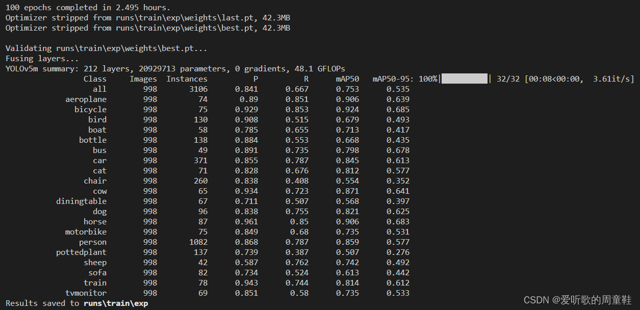
YOLOv5 训练效果如下图:
YOLOv6 训练效果如下图:
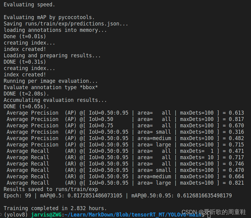
torch 的模型性能如下:
| Model | Size | mAPval 0.5:0.95 | mAPval 0.5 | Params (M) | FLOPs (G) |
|---|---|---|---|---|---|
| YOLOv5m | 640 | 53.5 | 75.3 | 21.2 | 49.0 |
| YOLOv6s | 640 | 61.3 | 81.7 | 18.5 | 45.3 |
2. TRT模型转换
pytorch 的模型已经训练好了,接下来我们就需要把 pytorch 训练好的模型导出为 onnx,然后让 tensorRT 通过 onnx 解析器去解析生成对应的 engine 文件。
值得注意的是本次测试过程中导出的 onnx 均为静态 batch,且 batch = 1
我们分别测试 FP32、FP16 以及 INT8 的性能
2.1 YOLOv5 ONNX导出
YOLOv5 模型的导出可参考 Ubuntu20.04部署YOLOv5
静态 batch 的 onnx 模型导出指令如下:
python export.py --weights=./runs/train/exp/weights/best.pt --include=onnx --opset=11
2.2 YOLOv6 ONNX导出
YOLOv6 模型的导出可参考 https://github.com/meituan/YOLOv6/tree/main/deploy/TensorRT
静态 batch 的 onnx 模型导出指令如下:
python ./deploy/ONNX/export_onnx.py --weights runs/train/exp/weights/best_ckpt.pt --img 640 --batch 1 --simplify
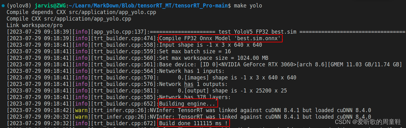
2.3 YOLOv5 engine生成
将导出的 onnx 利用 tensorRT 生成对应的 engine
YOLOv5 engine 的生成可参考 Ubuntu20.04部署YOLOv5
具体使用的是 tensorRT_Pro 这个 repo,简单修改下源码和 Makefile 文件后便可以构建 engine 模型了,这里不再赘述,更多细节请参考相关博文
模型构建如下图所示:
INT8 模型的构建由于使用的是 PTQ 量化,因此还需要准备校准数据集来计算量化参数,这次直接从训练集中随机抽取了 100 张图片进行校准。
关于 PTQ 量化的更多细节可参考:TensoRT量化第四课:PTQ与QAT
2.4 YOLOv6 engine生成
将导出的 onnx 利用 tensorRT 生成对应的 engine
YOLOv6 engine 的生成可参考 https://github.com/meituan/YOLOv6/tree/main/deploy/TensorRT
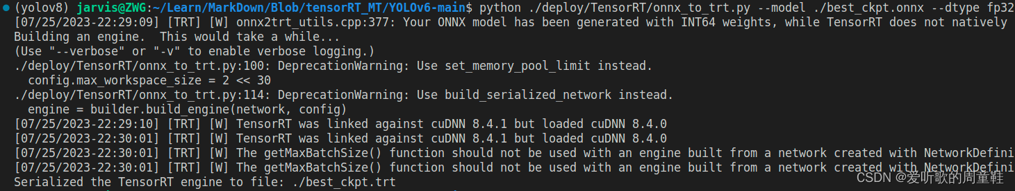
利用 tensorRT 的 Python API 生成 engine,具体指令如下:
python ./deploy/TensorRT/onnx_to_trt.py --model ./best_ckpt.onnx --dtype fp32/fp16 --verbose
出现如下问题:
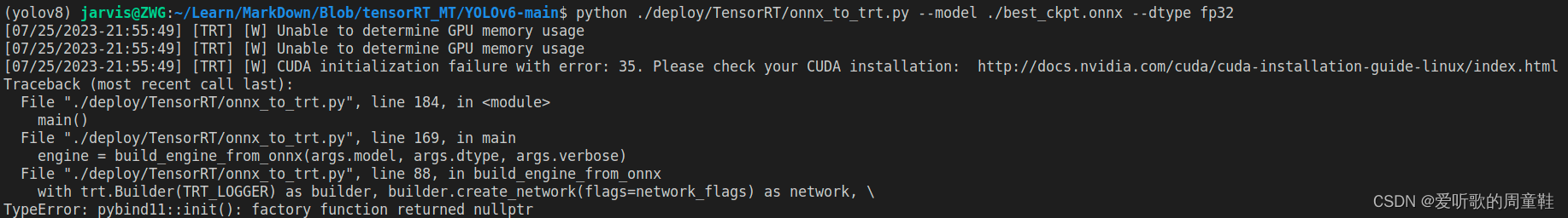
最后发现问题是 tensorrt 包默认安装的版本太高,为 8.6.1 版本,与我的环境不兼容,卸载后重新安装了一个低版本的就可以了,安装指令如下:
pip install tensorrt==8.5.1.7
模型构建如下图所示:
INT8 模型构建指令如下:
python ./deploy/TensorRT/onnx_to_trt.py --model ./best_ckpt.onnx --dtype int8 --calib-img-dir ./calib_data
YOLOv6 的 INT8 量化方式也是采取的 PTQ 量化,但是它规定了最少校准的图片需要 1000 张,因此博主从训练集中随机抽取了 1000 张作为样本图片。
3. TRT模型测试
TRT 模型拿到手后就可以愉快的进行测试了😏
本次 mAP 的测试和速度测试方法均参考自 tensorRT_Pro
3.1 YOLOv5 engine mAP测试
杜老师在 tensorRT_Pro 这个 repo 中提供了对应模型性能测试的代码,这次也主要是围绕杜老师提供的代码进行相关测试学习
mAP 测试代码地址:https://github.com/shouxieai/tensorRT_Pro/blob/main/src/application/test_yolo_map.cpp
代码需要我们提供一个图片文件夹路径,同时提供一个 TRT model,程序会利用 TRT model 在整个验证集上进行推理,我们会把模型推理的结果保存为 JSON 格式的文件,后续我们就可以拿着这个预测结果的 JSON 文件和我们真实标签的 JSON 文件通过 COCO Python API 去计算 mAP 指标.
mAP 测试代码如下:
#include <builder/trt_builder.hpp>
#include <infer/trt_infer.hpp>
#include <common/ilogger.hpp>
#include <common/json.hpp>
#include "app_yolo/yolo.hpp"
#include <vector>
#include <string>

using namespace std;

static const char *cocolabels[] = {"aeroplane",   "bicycle", "bird",   "boat",       "bottle",
                                  "bus",         "car",     "cat",    "chair",      "cow",
                                  "diningtable", "dog",     "horse",  "motorbike",  "person",
                                  "pottedplant",  "sheep",  "sofa",   "train",      "tvmonitor"};

bool requires(const char* name);

struct BoxLabel{
    int label;
    float cx, cy, width, height;
    float confidence;
};

struct ImageItem{
    string image_file;
    Yolo::BoxArray detections;
};

vector<ImageItem> scan_dataset(const string& images_root){

    vector<ImageItem> output;
    auto image_files = iLogger::find_files(images_root, "*.jpg");

    for(int i = 0; i < image_files.size(); ++i){
        auto& image_file = image_files[i];

        if(!iLogger::exists(image_file)){
            INFOW("Not found: %s", image_file.c_str());
            continue;
        }

        ImageItem item;
        item.image_file = image_file;
        output.emplace_back(item);
    }
    return output;
}

static void inference(vector<ImageItem>& images, int deviceid, const string& engine_file, TRT::Mode mode, Yolo::Type type, const string& model_name){

    INFO("===================== test Yolov5 INT8 best.sim ==================================");

    auto engine = Yolo::create_infer(
        engine_file, type, deviceid, 0.001f, 0.65f,
        Yolo::NMSMethod::CPU, 10000
    );
    if(engine == nullptr){
        INFOE("Engine is nullptr");
        return;
    }

    int nimages = images.size();
    vector<shared_future<Yolo::BoxArray>> image_results(nimages);
    for(int i = 0; i < nimages; ++i){
        if(i % 100 == 0){
            INFO("Commit %d / %d", i+1, nimages);
        }
        image_results[i] = engine->commit(cv::imread(images[i].image_file));
    }

    for(int i = 0; i < nimages; ++i)
        images[i].detections = image_results[i].get();
}

bool save_to_json(const vector<ImageItem>& images, const string& file){

    Json::Value predictions(Json::arrayValue);
    for(int i = 0; i < images.size(); ++i){
        auto& image = images[i];
        auto file_name = iLogger::file_name(image.image_file, false);
        string image_id = file_name;

        auto& boxes = image.detections;
        for(auto& box : boxes){
            Json::Value jitem;
            jitem["image_id"] = image_id;
            jitem["category_id"] = box.class_label;
            jitem["score"] = box.confidence;

            auto& bbox = jitem["bbox"];
            bbox.append(box.left);
            bbox.append(box.top);
            bbox.append(box.right - box.left);
            bbox.append(box.bottom - box.top);
            predictions.append(jitem);
        }
    }
    return iLogger::save_file(file, predictions.toStyledString());
}

int test_yolo_map(){

    /*
    结论:
    1. YoloV5在tensorRT下和pytorch下,只要输入一样,输出的差距最大值是1e-3
    2. YoloV5-6.0的mAP,官方代码跑下来是mAP@.5:.95 = 0.367, mAP@.5 = 0.554,与官方声称的有差距
    3. 这里的tensorRT版本测试的精度为:mAP@.5:.95 = 0.357, mAP@.5 = 0.539,与pytorch结果有差距
    4. cv2.imread与cv::imread,在操作jpeg图像时,在我这里测试读出的图像值不同,最大差距有19。而png图像不会有这个问题
        若想完全一致,请用png图像
    5. 预处理部分,若采用letterbox的方式做预处理,由于tensorRT这里是固定640x640大小,测试采用letterbox并把多余部分
        设置为0. 其推理结果与pytorch相近,但是依旧有差别
    6. 采用warpAffine和letterbox两种方式的预处理结果,在mAP上没有太大变化(小数点后三位差)
    7. mAP差一个点的原因可能在固定分辨率这件事上,还有是pytorch实现的所有细节并非完全加入进来。这些细节可能有没有
        找到的部分
    */

    auto images = scan_dataset("/home/jarvis/Learn/MarkDown/Blob/tensorRT_MT/dataset/images/val");
    INFO("images.size = %d", images.size());

    string model = "best.sim.INT8";
    inference(images, 0, "best.sim.INT8.trtmodel", TRT::Mode::INT8, Yolo::Type::V5, "best.sim.INT8");
    save_to_json(images, model + ".prediction.json");
    return 0;
}
上述代码的大体流程如下:
- 首先,程序扫描指定目录下的图像文件),将每个图像的文件路径保存到一个 ImageItem 实例中,形成一个图像列表。
- 接着,程序加载预先构建的 TensorRT 引擎,并使用该引擎对图像列表中的每个图像进行目标检测。
- 检测的结果(检测到的物体边界框和类别标签)被保存在对应的 ImageItem 实例中。
- 最后,程序将所有图像的检测结果存储到一个 JSON 文件中,每个检测到的物体都被序列化为 JSON 格式的信息(包括图像 ID、类别 ID、置信度和边界框坐标)。
主要有以下几点值得注意:
-
JSON 文件中 image_id 的保存为一个字符串,不再是整数,因为图片命名不一定是数值
-
JSON 文件中 category_id 的保存直接就是类别的标签,无需转换
-
mAP 测试使用的 NMS_threshold = 0.65f,Conf_threshold = 0.001f
-
关于 mAP 的相关原理介绍可参考 目标检测mAP计算以及coco评价标准
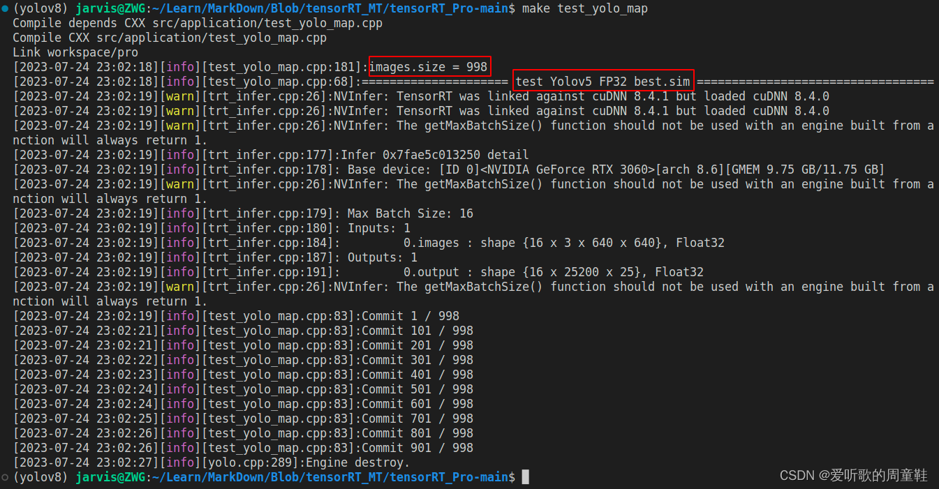
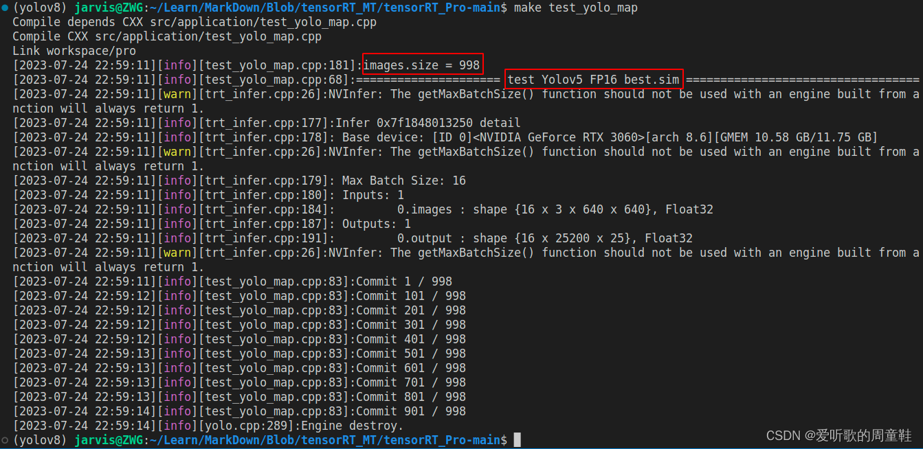
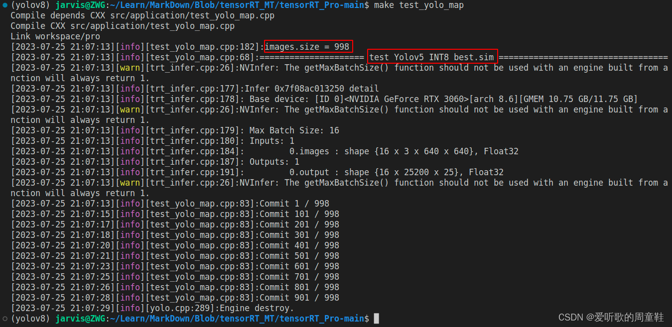
YOLOv5m engine 模型推理测试如下图所示:
经过 TRT model 的推理后就可以拿到预测结果的 JSON 文件了,除此之外我们还需要验证集真实标签的 JSON 文件,此时可以利用 1.4 小节的 yolo2json 将验证集的 YOLO 格式标签转换成 JSON 格式。
两个 JSON 文件都准备好了之后,我们就可以调用 COCO Python API 来进行 mAP 的测试了,具体代码如下:
from pycocotools.coco import COCO
from pycocotools.cocoeval import COCOeval

# Run COCO mAP evaluation
# Reference: https://github.com/cocodataset/cocoapi/blob/master/PythonAPI/pycocoEvalDemo.ipynb

annotations_path = "/home/jarvis/project/YOLOv6-3/tools/val.json"
results_file = "../result/prediction.json"
cocoGt = COCO(annotation_file=annotations_path)
cocoDt = cocoGt.loadRes(results_file)
imgIds = sorted(cocoGt.getImgIds())
cocoEval = COCOeval(cocoGt, cocoDt, 'bbox')
cocoEval.params.imgIds = imgIds
cocoEval.evaluate()
cocoEval.accumulate()
cocoEval.summarize()
你需要修改:
- annotations_path:验证集真实标签的 JSON 文件路径
- results_file:TRT model 预测结果的 JSON 文件路径
YOLOv5m engien 的 mAP 测试结果如下图:
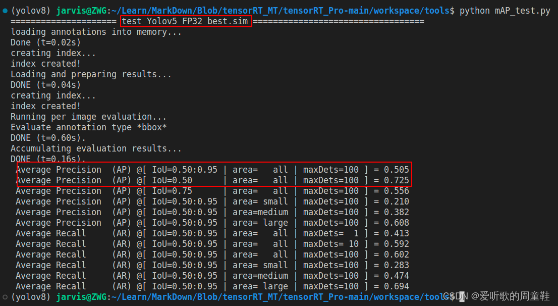
可以看到相比于原始 pytorch 的 mAP 指标而言(mAP50-95=0.535,mAP50=0.753),FP32 模型下降了 3 个点,一般来说 FP32 的 mAP 应该和 pytorch 的 mAP 接近,差了将近 3 个点可能是在预处理固定分辨率这件事情上,tensorRT_Pro 为了完成 warpAffine 加速,将图像固定在 640x640 的分辨率上。
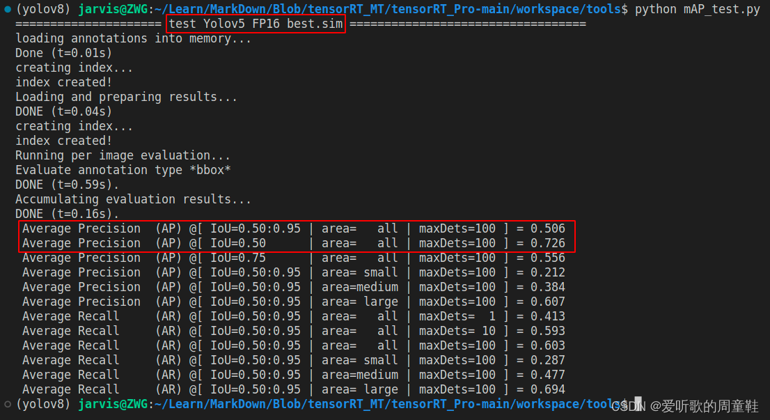
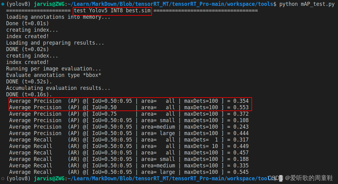
FP16 倒是没啥问题,相比于 FP32 无掉点。不过 INT8 掉点就有点大了,掉了将近 20 个点,后续博主在测试 YOLOv6s 的时候发现 INT8 也没有这么离谱吖,同样是 PTQ 量化,后面发现可能是标定图的数量缘故,在 YOLOv5m INT8 量化的时候校准图只准备了 100 张,而 YOLOv6s INT8 量化的时候则准备了 1000 张,因此博主把这 1000 张图片也拿过来给 YOLOv5m 校准了,测试结果如下:
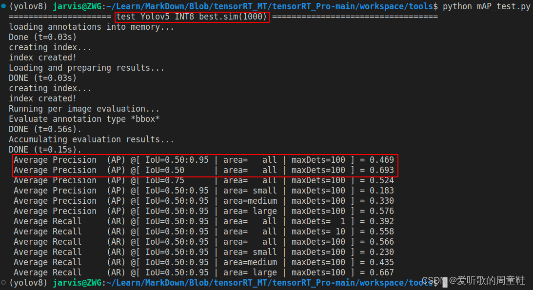
哇😍,可以看到效果得到了非常大的改善,相比于 100 张校准图涨了将近 14 个点,看来标定图片的数量对结果影响还是很大的。
总结下 YOLOv5m 的 mAP 测试结果,如下表所示:
| 模型名称 | 分辨率 | 精度 | mAPval 0.5:0.95 | mAPval 0.5 |
|---|---|---|---|---|
| YOLOv5m | 640 | - | 53.5 | 75.3 |
| YOLOv5m | 640 | FP32 | 50.5 | 72.5 |
| YOLOv5m | 640 | FP16 | 50.6 | 72.6 |
| YOLOv5m | 640 | INT8(100) | 35.4 | 55.3 |
| YOLOv5m | 640 | INT8(1000) | 46.9 | 69.3 |
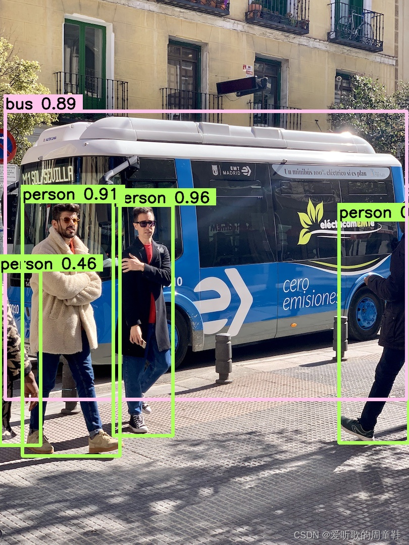
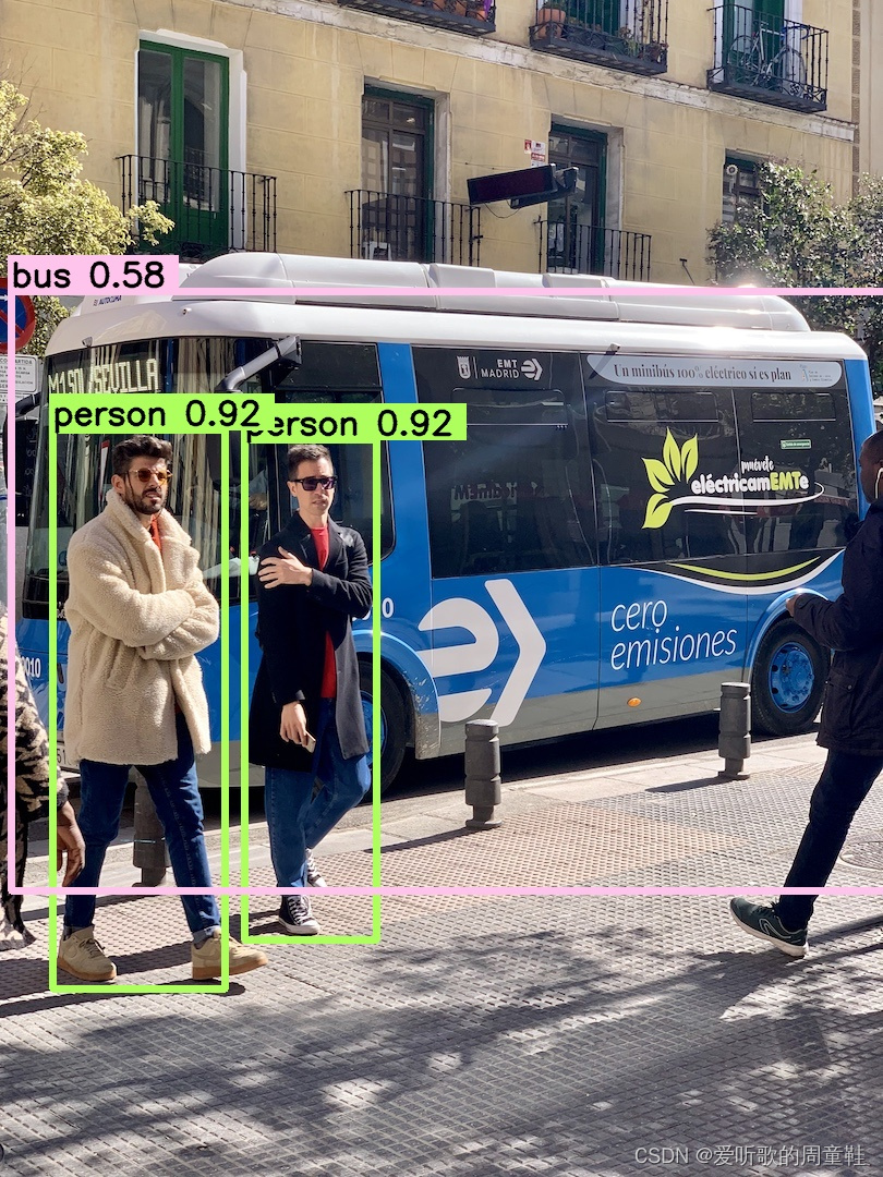
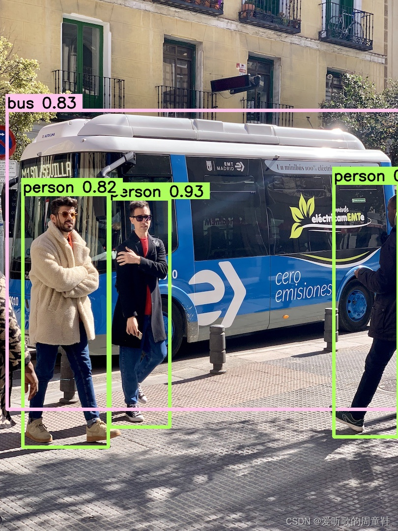
我找了一幅检测效果图,来对比看看不同精度下 TRT model 的检测效果:

3.2 YOLOv5 engine 速度测试
杜老师在 tensorRT_Pro 这个 repo 中提供了对应模型速度测试的代码,这次也主要是围绕杜老师提供的代码进行相关测试学习
速度测试代码地址:https://github.com/shouxieai/tensorRT_Pro/blob/main/src/application/app_yolo.cpp
关于 app_yolo.cpp 速度测试的说明:(from 杜老师)
1. 输入分辨率 640x640
2. batch size = 1
3. 图像预处理 + 推理 + 后处理
4. CUDA11.6,cuDNN8.4.0,TensorRT8.4.1.5
5. NVIDIA RTX3060
6. 测试次数,100 次取平均,去掉 warmup
7. 测试图像,6张。目录 workspace/inference
- 分辨率分别为:810x1080,500x806,1024x684,550x676,1280x720,800x533
8. 测试方式,加载 6 张图后,以原图重复 100 次不停塞进去。让模型经历完整的图像的预处理,后处理
YOLOv5 engine 模型速度测试结果如下图所示:
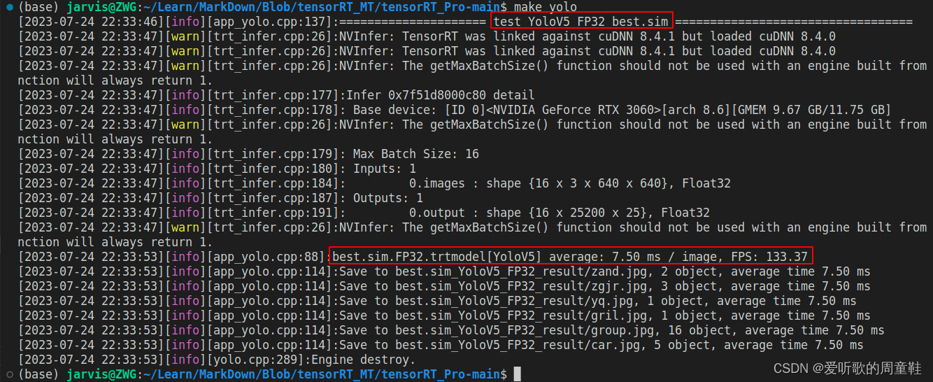
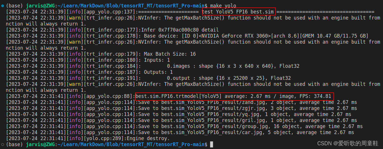
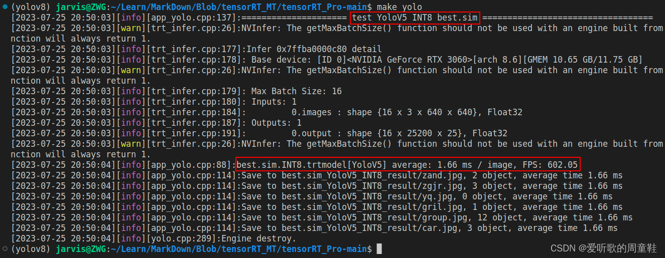
总结下 YOLOv5m 的速度测试结果,如下表所示:
| 模型名称 | 分辨率 | 精度 | 耗时/ms | 帧率/FPS |
|---|---|---|---|---|
| YOLOv5m | 640 | FP32 | 7.50 | 133.37 |
| YOLOv5m | 640 | FP16 | 2.67 | 374.81 |
| YOLOv5m | 640 | INT8 | 1.66 | 602.05 |
3.3 YOLOv6 engine mAP测试
YOLOv6 的 mAP 测试就是参考杜老师实现的,无非是把 YOLOv6 engine 推理的结果保存为 JSON,调用 COCO Python API 测试,这次我们自己来学习杜老师构建 YOLOv6 engine 测试项目,创建一个文件夹,目录结构如下所示:
YOLOv6_test
├─CMakeLists.txt
│
├─src
│  │  logging.h
│  │  main.cpp
│  │
│  └─common
│          ilogger.cpp
│          ilogger.hpp
│          json.cpp
│          json.hpp
│
└─workspace
src 文件夹下存放着所有源代码,其中 logging.h 和 main.cpp 来自于 https://github.com/meituan/YOLOv6/tree/main/deploy/TensorRT 的 logging.h 和 yolov6.cpp
logging.h 文件无修改,而 main.cpp 经过了修改,具体修改内容下面会提到
common 文件夹下存放着一些通用的工具文件主要用于日志输出和 JSON 文件的解析,其代码来自于 https://github.com/shouxieai/tensorRT_Pro/tree/main/src/tensorRT/common
workspace 文件夹下可用于存放编译好的可执行文件,以及模型文件,测试图片文件,保存的 JSON 文件等等
其中 CMakeLists.txt 文件用于编译,其内容如下:
cmake_minimum_required(VERSION 2.6)
project(pro)

add_definitions(-std=c++11)

option(CUDA_USE_STATIC_CUDA_RUNTIME OFF)
set(CMAKE_CXX_STANDARD 11)
set(CMAKE_BUILD_TYPE Debug)
set(EXECUTABLE_OUTPUT_PATH ${PROJECT_SOURCE_DIR}/workspace)
# add_definitions("-Wall -g")

set(OpenCV_DIR "/usr/local/")
set(CUDA_TOOLKIT_ROOT_DIR "/usr/local/cuda-11.6")
set(TENSORRT_DIR "/opt/TensorRT-8.4.1.5/")
find_package(CUDA REQUIRED)

# include and link dirs of cuda and tensorrt, you need adapt them if yours are different
include_directories(
    ${PROJECT_SOURCE_DIR}/src
    ${PROJECT_SOURCE_DIR}/src/common
    ${CUDA_TOOLKIT_ROOT_DIR}/include
    ${TENSORRT_DIR}/include
    ${OpenCV_DIR}/include/opencv4)


link_directories(
    ${CUDA_TOOLKIT_ROOT_DIR}/lib64
    ${TENSORRT_DIR}/lib
    ${OpenCV_DIR}/lib)

set(CMAKE_CXX_FLAGS "${CMAKE_CXX_FLAGS} -std=c++11 -Wall -Ofast -Wfatal-errors -pthread -D_MWAITXINTRIN_H_INCLUDED")
file(GLOB_RECURSE cpp_srcs ${PROJECT_SOURCE_DIR}/src/*.cpp)

add_executable(pro ${cpp_srcs})

target_link_libraries(pro pthread)
target_link_libraries(pro nvinfer)
target_link_libraries(pro cudart cudnn)
target_link_libraries(pro opencv_core opencv_imgproc opencv_highgui opencv_videoio opencv_imgcodecs)

add_definitions(-O2 -pthread)
你需要修改的是:
- 12行:OpenCV 的路径指定
- 13行:CUDA 的路径指定
- 14行:TensorRT 的路径指定
首先 main.cpp 中你需要修改下检测的类别数目以及输入和输出的名字:
const int num_class = 20;
static const int INPUT_W = 640;
static const int INPUT_H = 640;
const char* INPUT_BLOB_NAME = "images";
const char* OUTPUT_BLOB_NAME = "outputs";
static const char* class_names[] = {
        "aeroplane", "bicycle", "bird", "boat", "bottle", "bus", "car", "cat", "chair", "cow",
        "diningtable", "dog", "horse", "motorbike", "person", "pottedplant", "sheep", "sofa", "train", "tvmonitor"
    };
然后模仿上面 YOLOv5m engine 测试代码创建一个结构体用于存放图片路径和预测的结果:
struct Object
{
    cv::Rect_<float> rect;
    int label;
    float prob;
};

struct ImageItem{
    string image_file;
    std::vector<Object> detections;
};
然后定义 scan_dataset 函数用于获取所有需要测试的图片路径:
vector<ImageItem> scan_dataset(const string& images_root){

    vector<ImageItem> output;
    auto image_files = iLogger::find_files(images_root, "*.jpg");

    for(int i = 0; i < image_files.size(); ++i){
        auto& image_file = image_files[i];

        if(!iLogger::exists(image_file)){
            INFOW("Not found: %s", image_file.c_str());
            continue;
        }

        ImageItem item;
        item.image_file = image_file;
        output.emplace_back(item);
    }
    return output;
}
接下来就是 detect_images 函数用于模型的推理:
void detect_images(vector<ImageItem>& images, nvinfer1::IExecutionContext& context, const int& output_size){

    static float* prob = new float[output_size];

    int nimages = images.size();
    for(int i = 0; i < nimages; ++i){
        if(i % 100 == 0){
            INFO("Commit %d / %d", i + 1, nimages);
        }

        // 预处理
        auto image = images[i].image_file;
        cv::Mat img = cv::imread(image);
        int img_w = img.cols;
        int img_h = img.rows;
        cv::Mat pr_img = static_resize(img);
        // INFO("blob image");

        float* blob = blobFromImage(pr_img);
        float scale = std::min(INPUT_W / (img.cols*1.0), INPUT_H / (img.rows*1.0));

        // 推理
        doInference(context, blob, prob, output_size, pr_img.size());

        // 后处理
        decode_outputs(prob, output_size, images[i].detections, scale, img_w, img_h);

        // draw_objects(img, images[i].detections, image);
    }
}
最后通过 save_to_json 函数将上面推理的结果保存到 json 文件中:
bool save_to_json(const vector<ImageItem>& images, const string& file){

    INFO("begin save to json.");
    Json::Value predictions(Json::arrayValue);
    for(int i = 0; i < images.size(); ++i){
        auto& image = images[i];
        auto file_name = iLogger::file_name(image.image_file, false);
        // int image_id = atoi(file_name.c_str());

        auto& boxes = image.detections;
        for(auto& box : boxes){
            Json::Value jitem;
            jitem["image_id"] = file_name;
            jitem["category_id"] = box.label;

            auto& bbox = jitem["bbox"];
            bbox.append(roundFloat(box.rect.x, 3));
            bbox.append(roundFloat(box.rect.y, 3));
            bbox.append(roundFloat(box.rect.width, 3));
            bbox.append(roundFloat(box.rect.height,3));

            jitem["score"] = roundFloat(box.prob, 5);
            predictions.append(jitem);
        }
    }

    return iLogger::save_file(file, predictions.toStyledString());
}
完整的 main.cpp 的示例代码如下:
#include <fstream>
#include <iostream>
#include <sstream>
#include <numeric>
#include <chrono>
#include <vector>
#include <opencv2/opencv.hpp>
#include <dirent.h>
#include "NvInfer.h"
#include "cuda_runtime_api.h"
#include "logging.h"
#include "common/json.hpp"
#include "common/ilogger.hpp"
#include <cmath>

#define CHECK(status) \
    do\
    {\
        auto ret = (status);\
        if (ret != 0)\
        {\
            std::cerr << "Cuda failure: " << ret << std::endl;\
            abort();\
        }\
    } while (0)

#define DEVICE 0  // GPU id
#define NMS_THRESH 0.65
#define BBOX_CONF_THRESH 0.001

using namespace nvinfer1;
using namespace std;

// stuff we know about the network and the input/output blobs
const int num_class = 20;
static const int INPUT_W = 640;
static const int INPUT_H = 640;     // 384 or 640
const char* INPUT_BLOB_NAME = "images";
const char* OUTPUT_BLOB_NAME = "outputs";
static const char* class_names[] = {"aeroplane",   "bicycle", "bird",   "boat",       "bottle",
                                  "bus",         "car",     "cat",    "chair",      "cow",
                                  "diningtable", "dog",     "horse",  "motorbike",  "person",
                                  "pottedplant",  "sheep",  "sofa",   "train",      "tvmonitor"};

static Logger gLogger;

float roundFloat(float value, int decimalPlaces) {
    float multiplier = std::pow(10, decimalPlaces);
    float roundedValue = std::round(value * multiplier) / multiplier;
    return roundedValue;
}

cv::Mat static_resize(cv::Mat& img) {
    float r = std::min(INPUT_W / (img.cols*1.0), INPUT_H / (img.rows*1.0));
    int unpad_w = r * img.cols;
    int unpad_h = r * img.rows;
    cv::Mat re(unpad_h, unpad_w, CV_8UC3);
    cv::resize(img, re, re.size());
    cv::Mat out(INPUT_H, INPUT_W, CV_8UC3, cv::Scalar(114, 114, 114));
    re.copyTo(out(cv::Rect(0, 0, re.cols, re.rows)));
    return out;
}

struct Object
{
    cv::Rect_<float> rect;
    int label;
    float prob;
};


static inline float intersection_area(const Object& a, const Object& b)
{
    cv::Rect_<float> inter = a.rect & b.rect;
    return inter.area();
}

static void qsort_descent_inplace(std::vector<Object>& faceobjects, int left, int right)
{
    int i = left;
    int j = right;
    float p = faceobjects[(left + right) / 2].prob;

    while (i <= j)
    {
        while (faceobjects[i].prob > p)
            i++;

        while (faceobjects[j].prob < p)
            j--;

        if (i <= j)
        {
            // swap
            std::swap(faceobjects[i], faceobjects[j]);

            i++;
            j--;
        }
    }

    #pragma omp parallel sections
    {
        #pragma omp section
        {
            if (left < j) qsort_descent_inplace(faceobjects, left, j);
        }
        #pragma omp section
        {
            if (i < right) qsort_descent_inplace(faceobjects, i, right);
        }
    }
}

static void qsort_descent_inplace(std::vector<Object>& objects)
{
    if (objects.empty())
        return;

    qsort_descent_inplace(objects, 0, objects.size() - 1);
}

static void nms_sorted_bboxes(const std::vector<Object>& faceobjects, std::vector<int>& picked, float nms_threshold)
{
    picked.clear();

    const int n = faceobjects.size();

    std::vector<float> areas(n);
    for (int i = 0; i < n; i++)
    {
        areas[i] = faceobjects[i].rect.area();
    }

    for (int i = 0; i < n; i++)
    {
        const Object& a = faceobjects[i];

        int keep = 1;
        for (int j = 0; j < (int)picked.size(); j++)
        {
            const Object& b = faceobjects[picked[j]];

            // intersection over union
            float inter_area = intersection_area(a, b);
            float union_area = areas[i] + areas[picked[j]] - inter_area;
            // float IoU = inter_area / union_area
            if (inter_area / union_area > nms_threshold)
                keep = 0;
        }

        if (keep)
            picked.push_back(i);
    }
}


static void generate_yolo_proposals(float* feat_blob, int output_size, float prob_threshold, std::vector<Object>& objects)
{
    auto dets = output_size / (num_class + 5);
    for (int boxs_idx = 0; boxs_idx < dets; boxs_idx++)
    {
        const int basic_pos = boxs_idx *(num_class + 5);
        float x_center = feat_blob[basic_pos+0];
        float y_center = feat_blob[basic_pos+1];
        float w = feat_blob[basic_pos+2];
        float h = feat_blob[basic_pos+3];
        float x0 = x_center - w * 0.5f;
        float y0 = y_center - h * 0.5f;
        float box_objectness = feat_blob[basic_pos+4];
        // std::cout<<*feat_blob<<std::endl;
        for (int class_idx = 0; class_idx < num_class; class_idx++)
        {
            float box_cls_score = feat_blob[basic_pos + 5 + class_idx];
            float box_prob = box_objectness * box_cls_score;
            if (box_prob > prob_threshold)
            {
                Object obj;
                obj.rect.x = x0;
                obj.rect.y = y0;
                obj.rect.width = w;
                obj.rect.height = h;
                obj.label = class_idx;
                obj.prob = box_prob;

                objects.push_back(obj);
            }

        } // class loop
    }

}

float* blobFromImage(cv::Mat& img){
    cv::cvtColor(img, img, cv::COLOR_BGR2RGB);

    float* blob = new float[img.total()*3];
    int channels = 3;
    int img_h = img.rows;
    int img_w = img.cols;
    for (size_t c = 0; c < channels; c++)
    {
        for (size_t  h = 0; h < img_h; h++)
        {
            for (size_t w = 0; w < img_w; w++)
            {
                blob[c * img_w * img_h + h * img_w + w] =
                    (((float)img.at<cv::Vec3b>(h, w)[c]) / 255.0f);
            }
        }
    }
    return blob;
}


static void decode_outputs(float* prob, int output_size, std::vector<Object>& objects, float scale, const int img_w, const int img_h) {
        std::vector<Object> proposals;
        generate_yolo_proposals(prob, output_size, BBOX_CONF_THRESH, proposals);
        // INFO("num of boxes before nms: %d", proposals.size());

        qsort_descent_inplace(proposals);

        std::vector<int> picked;
        nms_sorted_bboxes(proposals, picked, NMS_THRESH);

        int count = picked.size();

        // INFO("num of boxes: %d", count);

        // INFO("conf_thresh =  %.2f, nms_thresh = %.2f", BBOX_CONF_THRESH, NMS_THRESH);
        objects.resize(count);
        for (int i = 0; i < count; i++)
        {
            objects[i] = proposals[picked[i]];

            // adjust offset to original unpadded
            float x0 = (objects[i].rect.x) / scale;
            float y0 = (objects[i].rect.y) / scale;
            float x1 = (objects[i].rect.x + objects[i].rect.width) / scale;
            float y1 = (objects[i].rect.y + objects[i].rect.height) / scale;

            // clip
            x0 = std::max(std::min(x0, (float)(img_w - 1)), 0.f);
            y0 = std::max(std::min(y0, (float)(img_h - 1)), 0.f);
            x1 = std::max(std::min(x1, (float)(img_w - 1)), 0.f);
            y1 = std::max(std::min(y1, (float)(img_h - 1)), 0.f);

            objects[i].rect.x = x0;
            objects[i].rect.y = y0;
            objects[i].rect.width = x1 - x0;
            objects[i].rect.height = y1 - y0;
        }
}

const float color_list[80][3] =
{
    {0.000, 0.447, 0.741},
    {0.850, 0.325, 0.098},
    {0.929, 0.694, 0.125},
    {0.494, 0.184, 0.556},
    {0.466, 0.674, 0.188},
    {0.301, 0.745, 0.933},
    {0.635, 0.078, 0.184},
    {0.300, 0.300, 0.300},
    {0.600, 0.600, 0.600},
    {1.000, 0.000, 0.000},
    {1.000, 0.500, 0.000},
    {0.749, 0.749, 0.000},
    {0.000, 1.000, 0.000},
    {0.000, 0.000, 1.000},
    {0.667, 0.000, 1.000},
    {0.333, 0.333, 0.000},
    {0.333, 0.667, 0.000},
    {0.333, 1.000, 0.000},
    {0.667, 0.333, 0.000},
    {0.667, 0.667, 0.000},
    {0.667, 1.000, 0.000},
    {1.000, 0.333, 0.000},
    {1.000, 0.667, 0.000},
    {1.000, 1.000, 0.000},
    {0.000, 0.333, 0.500},
    {0.000, 0.667, 0.500},
    {0.000, 1.000, 0.500},
    {0.333, 0.000, 0.500},
    {0.333, 0.333, 0.500},
    {0.333, 0.667, 0.500},
    {0.333, 1.000, 0.500},
    {0.667, 0.000, 0.500},
    {0.667, 0.333, 0.500},
    {0.667, 0.667, 0.500},
    {0.667, 1.000, 0.500},
    {1.000, 0.000, 0.500},
    {1.000, 0.333, 0.500},
    {1.000, 0.667, 0.500},
    {1.000, 1.000, 0.500},
    {0.000, 0.333, 1.000},
    {0.000, 0.667, 1.000},
    {0.000, 1.000, 1.000},
    {0.333, 0.000, 1.000},
    {0.333, 0.333, 1.000},
    {0.333, 0.667, 1.000},
    {0.333, 1.000, 1.000},
    {0.667, 0.000, 1.000},
    {0.667, 0.333, 1.000},
    {0.667, 0.667, 1.000},
    {0.667, 1.000, 1.000},
    {1.000, 0.000, 1.000},
    {1.000, 0.333, 1.000},
    {1.000, 0.667, 1.000},
    {0.333, 0.000, 0.000},
    {0.500, 0.000, 0.000},
    {0.667, 0.000, 0.000},
    {0.833, 0.000, 0.000},
    {1.000, 0.000, 0.000},
    {0.000, 0.167, 0.000},
    {0.000, 0.333, 0.000},
    {0.000, 0.500, 0.000},
    {0.000, 0.667, 0.000},
    {0.000, 0.833, 0.000},
    {0.000, 1.000, 0.000},
    {0.000, 0.000, 0.167},
    {0.000, 0.000, 0.333},
    {0.000, 0.000, 0.500},
    {0.000, 0.000, 0.667},
    {0.000, 0.000, 0.833},
    {0.000, 0.000, 1.000},
    {0.000, 0.000, 0.000},
    {0.143, 0.143, 0.143},
    {0.286, 0.286, 0.286},
    {0.429, 0.429, 0.429},
    {0.571, 0.571, 0.571},
    {0.714, 0.714, 0.714},
    {0.857, 0.857, 0.857},
    {0.000, 0.447, 0.741},
    {0.314, 0.717, 0.741},
    {0.50, 0.5, 0}
};


static void draw_objects(const cv::Mat& bgr, const std::vector<Object>& objects, std::string f)
{

    cv::Mat image = bgr.clone();

    for (size_t i = 0; i < objects.size(); i++)
    {
        const Object& obj = objects[i];

        fprintf(stderr, "%d = %.5f at %.2f %.2f %.2f x %.2f\n", obj.label, obj.prob,
                obj.rect.x, obj.rect.y, obj.rect.width, obj.rect.height);

        cv::Scalar color = cv::Scalar(color_list[obj.label][0], color_list[obj.label][1], color_list[obj.label][2]);
        float c_mean = cv::mean(color)[0];
        cv::Scalar txt_color;
        if (c_mean > 0.5){
            txt_color = cv::Scalar(0, 0, 0);
        }else{
            txt_color = cv::Scalar(255, 255, 255);
        }

        cv::rectangle(image, obj.rect, color * 255, 2);

        char text[256];
        sprintf(text, "%s %.1f%%", class_names[obj.label], obj.prob * 100);

        int baseLine = 0;
        cv::Size label_size = cv::getTextSize(text, cv::FONT_HERSHEY_SIMPLEX, 0.4, 1, &baseLine);

        cv::Scalar txt_bk_color = color * 0.7 * 255;

        int x = obj.rect.x;
        int y = obj.rect.y + 1;
        //int y = obj.rect.y - label_size.height - baseLine;
        if (y > image.rows)
            y = image.rows;
        //if (x + label_size.width > image.cols)
            //x = image.cols - label_size.width;

        cv::rectangle(image, cv::Rect(cv::Point(x, y), cv::Size(label_size.width, label_size.height + baseLine)),
                      txt_bk_color, -1);

        cv::putText(image, text, cv::Point(x, y + label_size.height),
                    cv::FONT_HERSHEY_SIMPLEX, 0.4, txt_color, 1);
    }

    cv::imwrite("result.jpg", image);
    fprintf(stderr, "save vis file\n");
    /* cv::imshow("image", image); */
    /* cv::waitKey(0); */
}


void doInference(IExecutionContext& context, float* input, float* output, const int output_size, cv::Size input_shape) {
    const ICudaEngine& engine = context.getEngine();

    // Pointers to input and output device buffers to pass to engine.
    // Engine requires exactly IEngine::getNbBindings() number of buffers.
    assert(engine.getNbBindings() == 2);
    void* buffers[2];

    // In order to bind the buffers, we need to know the names of the input and output tensors.
    // Note that indices are guaranteed to be less than IEngine::getNbBindings()
    const int inputIndex = engine.getBindingIndex(INPUT_BLOB_NAME);

    assert(engine.getBindingDataType(inputIndex) == nvinfer1::DataType::kFLOAT);
    const int outputIndex = engine.getBindingIndex(OUTPUT_BLOB_NAME);
    assert(engine.getBindingDataType(outputIndex) == nvinfer1::DataType::kFLOAT);
    // int mBatchSize = engine.getMaxBatchSize();

    // Create GPU buffers on device
    CHECK(cudaMalloc(&buffers[inputIndex], 3 * input_shape.height * input_shape.width * sizeof(float)));
    CHECK(cudaMalloc(&buffers[outputIndex], output_size*sizeof(float)));

    // Create stream
    cudaStream_t stream;
    CHECK(cudaStreamCreate(&stream));

    // DMA input batch data to device, infer on the batch asynchronously, and DMA output back to host
    CHECK(cudaMemcpyAsync(buffers[inputIndex], input, 3 * input_shape.height * input_shape.width * sizeof(float), cudaMemcpyHostToDevice, stream));
    // context.enqueue(1, buffers, stream, nullptr);
    context.enqueueV2(buffers, stream, nullptr);

    CHECK(cudaMemcpyAsync(output, buffers[outputIndex], output_size * sizeof(float), cudaMemcpyDeviceToHost, stream));
    cudaStreamSynchronize(stream);

    // Release stream and buffers
    cudaStreamDestroy(stream);
    CHECK(cudaFree(buffers[inputIndex]));
    CHECK(cudaFree(buffers[outputIndex]));
}


struct ImageItem{
    string image_file;
    std::vector<Object> detections;
};

vector<ImageItem> scan_dataset(const string& images_root){

    vector<ImageItem> output;
    auto image_files = iLogger::find_files(images_root, "*.jpg");

    for(int i = 0; i < image_files.size(); ++i){
        auto& image_file = image_files[i];

        if(!iLogger::exists(image_file)){
            INFOW("Not found: %s", image_file.c_str());
            continue;
        }

        ImageItem item;
        item.image_file = image_file;
        output.emplace_back(item);
    }
    return output;
}


void detect_images(vector<ImageItem>& images, nvinfer1::IExecutionContext& context, const int& output_size){

    static float* prob = new float[output_size];

    int nimages = images.size();
    for(int i = 0; i < nimages; ++i){
        if(i % 2 == 0){
            INFO("Commit %d / %d", i + 1, nimages);
        }

        // 预处理
        auto image = images[i].image_file;
        cv::Mat img = cv::imread(image);
        int img_w = img.cols;
        int img_h = img.rows;
        cv::Mat pr_img = static_resize(img);
        // INFO("blob image");

        float* blob = blobFromImage(pr_img);
        float scale = std::min(INPUT_W / (img.cols*1.0), INPUT_H / (img.rows*1.0));

        // 推理
        doInference(context, blob, prob, output_size, pr_img.size());

        // 后处理
        decode_outputs(prob, output_size, images[i].detections, scale, img_w, img_h);

        // draw_objects(img, images[i].detections, image);

    }

}

bool save_to_json(const vector<ImageItem>& images, const string& file){

    INFO("begin save to json.");
    Json::Value predictions(Json::arrayValue);
    for(int i = 0; i < images.size(); ++i){
        auto& image = images[i];
        auto file_name = iLogger::file_name(image.image_file, false);
        // int image_id = atoi(file_name.c_str());

        auto& boxes = image.detections;
        for(auto& box : boxes){
            Json::Value jitem;
            jitem["image_id"] = file_name;
            jitem["category_id"] = box.label;

            auto& bbox = jitem["bbox"];
            bbox.append(roundFloat(box.rect.x, 3));
            bbox.append(roundFloat(box.rect.y, 3));
            bbox.append(roundFloat(box.rect.width, 3));
            bbox.append(roundFloat(box.rect.height,3));

            jitem["score"] = roundFloat(box.prob, 5);
            predictions.append(jitem);
        }
    }

    return iLogger::save_file(file, predictions.toStyledString());
}

// ./pro best_640x640.trt -i imgs/xxx.jpg

void speed_test(nvinfer1::IExecutionContext& context, const int& output_size, const string& engine_file){

    auto files = iLogger::find_files("imgs", "*.jpg;*.jpeg;*.png;*.gif;*.tif");

    vector<cv::Mat> images;
    for(int i = 0; i < files.size(); ++i){
        auto image = cv::imread(files[i]);
        images.emplace_back(image);
    }

    static float* prob = new float[output_size];
    std::vector<Object> objects;

    // warm up
    for(int i = 0; i < 5; ++i){
        for(int j = 0; j < images.size(); ++j){
            cv::Mat img = images[j];
            int img_w = img.cols;
            int img_h = img.rows;
            float scale = std::min(INPUT_W / (img.cols*1.0), INPUT_H / (img.rows*1.0));

            cv::Mat pr_img = static_resize(img);
            float* blob = blobFromImage(pr_img);

            doInference(context, blob, prob, output_size, pr_img.size());

            decode_outputs(prob, output_size, objects, scale, img_w, img_h);

            // objects.clear();
        }
    }

    INFO("warm up done!");


    float count = 0;
    const int ntest = 10;

    for(int i = 0; i < ntest; ++i){
        for(int j = 0; j < images.size(); ++j){

            cv::Mat img = images[j];
            int img_w = img.cols;
            int img_h = img.rows;
            float scale = std::min(INPUT_W / (img.cols*1.0), INPUT_H / (img.rows*1.0));

            cv::Mat pr_img = static_resize(img);
            float* blob = blobFromImage(pr_img);

            auto begin_timer = iLogger::timestamp_now_float();

            doInference(context, blob, prob, output_size, pr_img.size());

            count += (iLogger::timestamp_now_float() - begin_timer);

            decode_outputs(prob, output_size, objects, scale, img_w, img_h);

            // objects.clear();
        }
    }

    float inference_average_time = count / ntest / images.size();

    INFO("%s average: %.2f ms / image, FPS = %.2f", engine_file.c_str(), inference_average_time, 1000 / inference_average_time);

}


int main(int argc, char** argv) {
    cudaSetDevice(DEVICE);
    // create a model using the API directly and serialize it to a stream
    char *trtModelStream{nullptr};
    size_t size{0};
    const std::string engine_file_path = "./best_ckpt-int8-128-6-minmax.trt" ;  // best_384x640.trt or best_640x640.trt
    std::ifstream file(engine_file_path, std::ios::binary);
    if (file.good()) {
        file.seekg(0, file.end);
        size = file.tellg();
        file.seekg(0, file.beg);
        trtModelStream = new char[size];
        assert(trtModelStream);
        file.read(trtModelStream, size);
        file.close();
    }

    IRuntime* runtime = createInferRuntime(gLogger);
    assert(runtime != nullptr);
    ICudaEngine* engine = runtime->deserializeCudaEngine(trtModelStream, size);
    assert(engine != nullptr);
    IExecutionContext* context = engine->createExecutionContext();
    assert(context != nullptr);
    delete[] trtModelStream;
    auto out_dims = engine->getBindingDimensions(1);
    auto output_size = 1;
    for(int j=0;j<out_dims.nbDims;j++) {
        output_size *= out_dims.d[j];
    }

    // 获取模型中所有绑定(输入和输出)的数量
    int numBindings = engine->getNbBindings();
    // 遍历所有绑定,并打印其名称和形状大小
    for (int i = 0; i < numBindings; ++i){
        std::string bingdingName   = engine->getBindingName(i);
        nvinfer1::Dims bindingDims = engine->getBindingDimensions(i);

        INFO("Binding Name: %s", bingdingName.c_str());
        std::cout << "Binding Shape: (";
        for (int j = 0; j < bindingDims.nbDims; j++) {
            std::cout << bindingDims.d[j];
            if (j < bindingDims.nbDims - 1) {
                std::cout << ", ";
            }
        }
        std::cout << ")" << std::endl;
    }
    INFO("INPUT_H = %d, engine_file = %s", INPUT_H, engine_file_path.c_str());


    // === speed test ===
    // INFO("begin speed test...");
    // speed_test(*context, output_size, engine_file_path);
    // INFO("speed test finised!!!");


    // === mAP test ===
    auto images = scan_dataset("/home/jarvis/Learn/MarkDown/Blob/tensorRT_MT/dataset/images/val");
    INFO("images.size = %d", images.size());
    detect_images(images, *context, output_size);
    save_to_json(images, "./v6_FP32.json");
    INFO("save done.");

    context->destroy();
    engine->destroy();
    runtime->destroy();
    return 0;
}
上述代码中 mAP 测试和 YOLOv5m 一致,detect_images 函数用于对输入图像进行推理和检测,将检测结果存储在 ImageItem 对象中。save_to_json 函数将检测结果以 JSON 格式保存到文件中。整体流程是,遍历图像集合,对每张图像进行预处理、推理和后处理得到检测结果,并将结果保存为 JSON 文件,以便后续的 mAP 计算和评估。
主要有以下几点值得注意:
- JSON 文件中 image_id 的保存为一个字符串,不再是整数,因为图片命名不一定是数值
- JSON 文件中 category_id 的保存直接就是类别的标签,无需转换
- mAP 测试使用的 NMS_threshold = 0.65f,Conf_threshold = 0.001f
- 关于 mAP 的相关原理介绍可参考 目标检测mAP计算以及coco评价标准
- 完整的代码可通过 here【pwd:yolo】 下载
YOLOv6s engine 模型推理测试如下图所示:
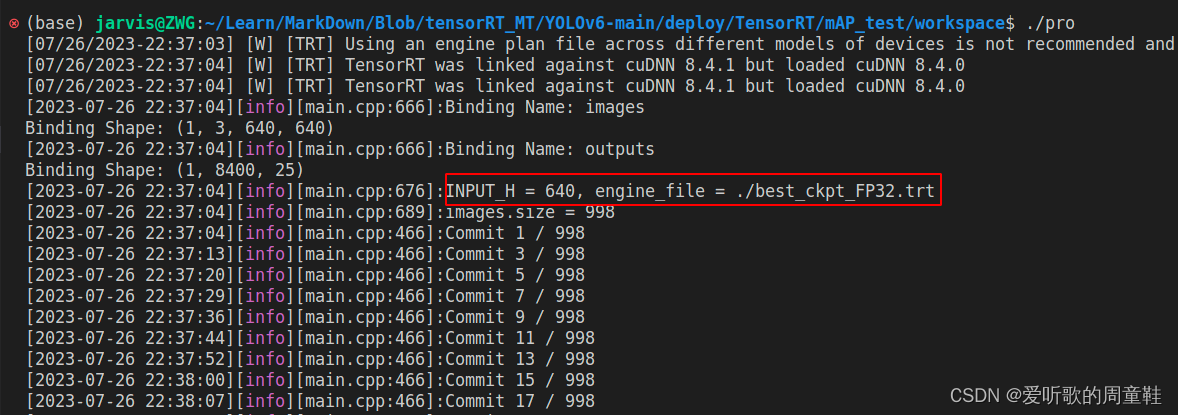
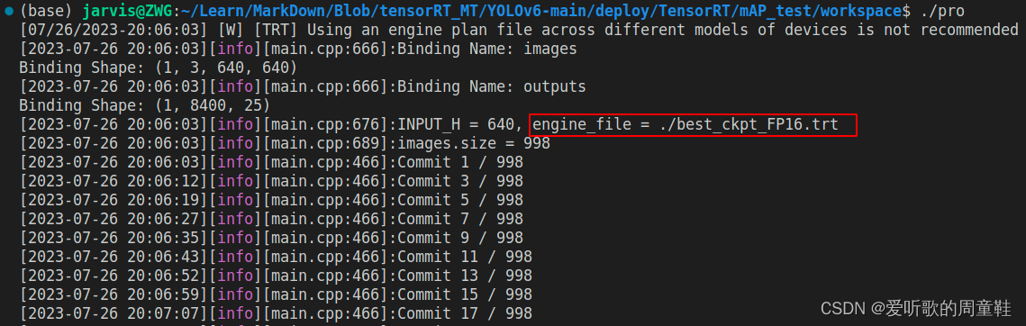
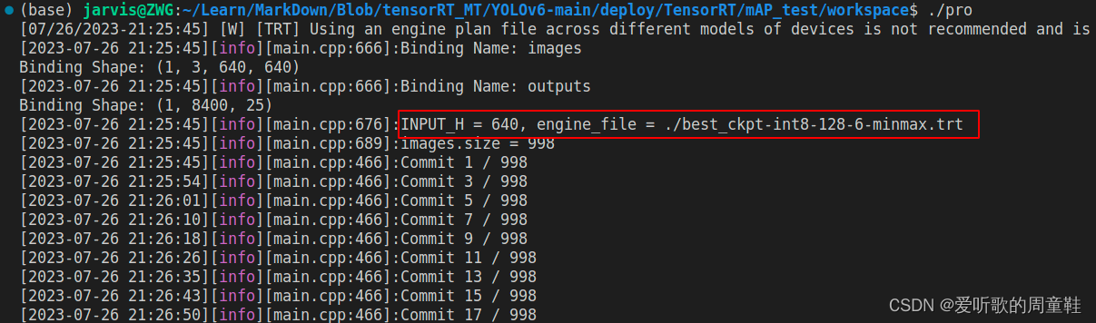
同理拿到 YOLOv6s TRT model 预测的 JSON 文件后,我们还需要真实标签的 JSON 文件,此时可以利用 1.4 小节的 yolo2json 将验证集的 YOLO 格式标签转换成 JSON 格式
两个 JSON 文件都有了,我们可以调用 COCO Python API 来进行 mAP 的测试了,具体代码如下:
from pycocotools.coco import COCO
from pycocotools.cocoeval import COCOeval

# Run COCO mAP evaluation
# Reference: https://github.com/cocodataset/cocoapi/blob/master/PythonAPI/pycocoEvalDemo.ipynb

print("===================== test Yolov6 INT8 best_ckpt ==================================")

annotations_path = "./val.json"
results_file = "./v6_INT8.json"
cocoGt = COCO(annotation_file=annotations_path)
cocoDt = cocoGt.loadRes(results_file)
imgIds = sorted(cocoGt.getImgIds())
cocoEval = COCOeval(cocoGt, cocoDt, 'bbox')
cocoEval.params.imgIds = imgIds
cocoEval.evaluate()
cocoEval.accumulate()
cocoEval.summarize()
你需要修改:
- annotations_path:验证集真实标签的 JSON 文件路径
- results_file:TRT model 预测结果的 JSON 文件路径
YOLOv6s engine 的 mAP 测试结果如下图:


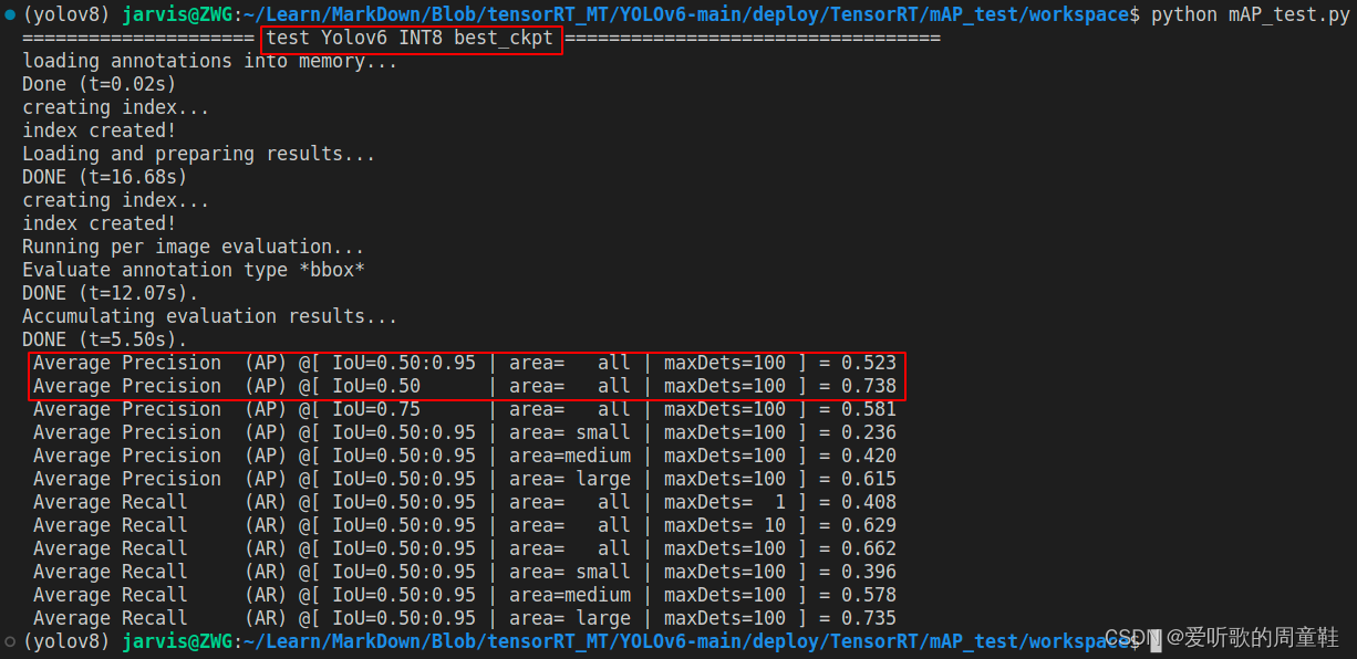
可以看到相比于原始 pytorch 的 mAP 指标而言(mAP50-95=0.613 mAP50=0.817),FP32 模型下降了 1.5 个点,比 YOLOv5m 下降得少,毕竟 YOLOv6s 的预处理方式和 pytorch 的保持一致。
FP16 模型与 FP32 性能相同,无掉点,INT8 模型掉了将近 8~9 个点
总结下 YOLOv6s 的 mAP 测试结果,如下表所示:
| 模型名称 | 分辨率 | 精度 | mAPval 0.5:0.95 | mAPval 0.5 |
|---|---|---|---|---|
| YOLOv6s | 640 | - | 61.3 | 81.7 |
| YOLOv6s | 640 | FP32 | 59.6 | 80.6 |
| YOLOv6s | 640 | FP16 | 59.6 | 80.5 |
| YOLOv6s | 640 | INT8 | 52.3 | 73.8 |
我找了一副检测效果图,来对比看看不同精度下 TRT model 的检测效果:
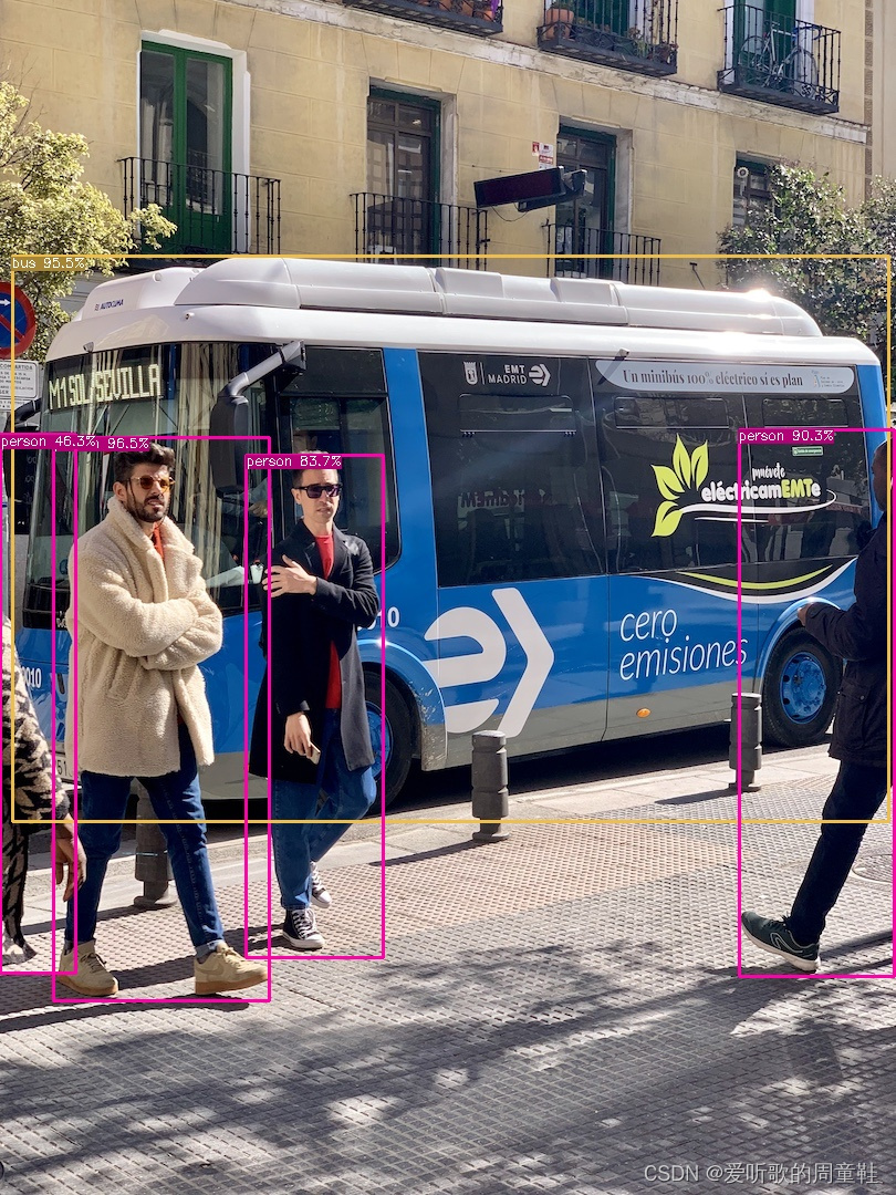


YOLOv6s INT8 的效果相比 YOLOv5m INT8 而言有点差咯,虽然一个个置信度很高但是误检有点多吖,而且误检置信度也高,通过置信度阈值也没办法剔除😂
3.4 YOLOv6 engine 速度测试
YOLOv6 的速度测试也是参考杜老师实现的
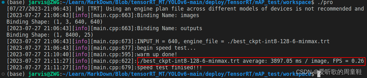
重点说明:由于预处理和后处理没有通过 CUDA 加速,所以各个不同精度的模型的推理速度完全看不出差别,同时由于 YOLOv6s 的推理是 demo 级别的,完全没办法和 tensorRT_Pro 这种工业级高性能推理框架相比,所以推理一张图的时间超慢。连 INT8 模型的一张图的预处理+推理+后处理都需要4s左右,如下图所示:
如果按照之前的 YOLOv5m 速度测试方法,加载 6 张图塞 100 次给模型推理,光是一个模型测试就花了博主将近 2 个小时,测出来发现 FP32、FP16 和 INT8 竟然毫无差别😱,我和我的小伙伴们都惊呆了
后面发现是预处理和后处理太耗时了,完全体现不出 FP32、FP16、INT8 模型的速度差距,因此 YOLOv6s 的速度测试我们需要改变下策略,我们只看推理速度,而不再考虑预处理和后处理。
而且由于预处理和后处理速度太慢,因此测试次数只取 10 次,测试图像还是 6 张,去掉 warmup
关于 YOLOv6s 速度测试的说明:(from 杜老师)
1. 输入分辨率 640x640
2. batch size = 1
3. 仅考虑推理
4. CUDA11.6,cuDNN8.4.0,TensorRT8.4.1.5
5. RTX3060
6. 测试次数,10 次取平均,去掉 warmup
7. 测试图像,6张。目录 workspace/inference
- 分辨率分别为:810x1080,500x806,1024x684,550x676,1280x720,800x533
8. 测试方式,加载 6 张图后,以原图重复 10 次不停塞进去。让模型经历完整的图像的预处理,后处理
用于速度测试的函数代码如下:
void speed_test(nvinfer1::IExecutionContext& context, const int& output_size, const string& engine_file){

    auto files = iLogger::find_files("imgs", "*.jpg;*.jpeg;*.png;*.gif;*.tif");

    vector<cv::Mat> images;
    for(int i = 0; i < files.size(); ++i){
        auto image = cv::imread(files[i]);
        images.emplace_back(image);
    }

    static float* prob = new float[output_size];
    std::vector<Object> objects;

    // warm up
    for(int i = 0; i < 5; ++i){
        for(int j = 0; j < images.size(); ++j){
            cv::Mat img = images[j];
            int img_w = img.cols;
            int img_h = img.rows;
            float scale = std::min(INPUT_W / (img.cols*1.0), INPUT_H / (img.rows*1.0));

            cv::Mat pr_img = static_resize(img);
            float* blob = blobFromImage(pr_img);

            doInference(context, blob, prob, output_size, pr_img.size());

            decode_outputs(prob, output_size, objects, scale, img_w, img_h);

            // objects.clear();
        }
    }

    INFO("warm up done!");


    float count = 0;
    const int ntest = 10;

    for(int i = 0; i < ntest; ++i){
        for(int j = 0; j < images.size(); ++j){

            cv::Mat img = images[j];
            int img_w = img.cols;
            int img_h = img.rows;
            float scale = std::min(INPUT_W / (img.cols*1.0), INPUT_H / (img.rows*1.0));

            cv::Mat pr_img = static_resize(img);
            float* blob = blobFromImage(pr_img);

            auto begin_timer = iLogger::timestamp_now_float();

            doInference(context, blob, prob, output_size, pr_img.size());

            count += (iLogger::timestamp_now_float() - begin_timer);

            decode_outputs(prob, output_size, objects, scale, img_w, img_h);

            // objects.clear();
        }
    }

    float inference_average_time = count / ntest / images.size();

    INFO("%s average: %.2f ms / image, FPS = %.2f", engine_file.c_str(), inference_average_time, 1000 / inference_average_time);

}
YOLOv6 engine 模型速度测试如下图所示:
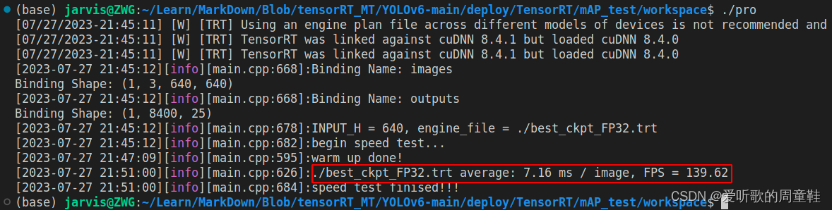
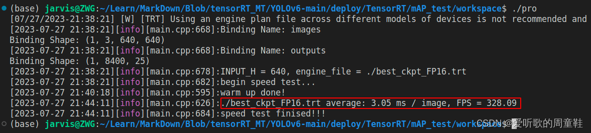
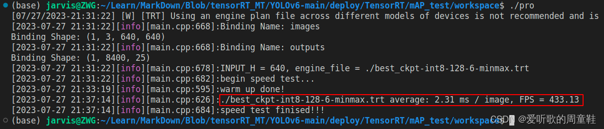
总结下 YOLOv6s 的速度测试结果,如下表所示:
| 模型名称 | 分辨率 | 精度 | 耗时/ms | 帧率/FPS |
|---|---|---|---|---|
| YOLOv6s | 640 | FP32 | 7.16 | 139.62 |
| YOLOv6s | 640 | FP16 | 3.05 | 382.09 |
| YOLOv6s | 640 | INT8 | 2.31 | 433.13 |
YOLOv5m 和 YOLOv6s 其实是两个参数差不多的模型,YOLOv5s FP32 模型测试的预处理+推理+后处理的时间是 7.50ms,YOLOv6s FP32 模型测试的预处理+推理+后处理的时间大概是 3897 ms,而推理时间是 7.16ms,意味着 YOLOv6s 预处理+后处理平均一张图花费了 3890 ms,这对比下来说明预处理和后处理的加速对于速度提升是非常重要的。
4. 讨论
讨论1:博主在这里只是简单通过这么一个流程测试了 TRT 模型的 mAP 和 速度,最主要的是分享测试的方法,仅供参考,思路就是这么一个思路,各位看官也可以自行编写相关代码实现,无非是保存 TRT 推理的结果和实际的真实结果进行比较得出 mAP,那可以看到无论是 YOLOv5 模型还是 YOLOv6 模型其 FP32 和 FP16 的模型精度并没有太大变化,那测试 mAP 真正用途感觉还是拿去测试 INT8 模型量化后的掉点情况。
讨论2:关于上述测量结果仅作参考,博主还只仅仅测试了静态 batch 模型,并没有去测试动态 batch,同时 YOLOv6 推理的代码是 demo 级别的,其 tensorRT 还是使用的 enqueue 而不是 enqueueV2,我们的目的只是为了简单测试 tensorRT 模型的性能,把整体流程走一遍,所以有些地方没有那么严谨。此外,关于速度的测试是存在波动的,毕竟到了 ms 级别,偶尔有些偏差也正常
讨论3:在模型实际应用过程中,我们并不能光看 mAP 一个指标就判断一个模型的优劣,YOLOv6s INT8 模型精度虽然比 YOLOv5m INT8 模型精度高了 4 个点,但是实际推理测试的结果还不如 YOLOv5m INT8,对比图 3-11 和图 3-23 可以发现,YOLOv6s INT8 模型存在许多高置信度的误检,这是我们不太希望看到的。因此评价一个模型需要综合考虑虚警率,误检率等多项指标才行。
我们来统一看下 YOLOv5 和 YOLOv6 模型性能测试结果:
| 模型名称 | 分辨率 | 精度 | mAPval 0.5:0.95 | mAPval 0.5 | 耗时/ms | 帧率/FPS |
|---|---|---|---|---|---|---|
| YOLOv5m | 640 | - | 53.5 | 75.3 | - | - |
| YOLOv5m | 640 | FP32 | 50.5 | 72.5 | 7.50 | 133.37 |
| YOLOv5m | 640 | FP16 | 50.6 | 72.6 | 2.67 | 374.81 |
| YOLOv5m | 640 | INT8 | 46.9 | 69.3 | 1.66 | 602.05 |
| YOLOv6s | 640 | - | 61.3 | 81.7 | - | - |
| YOLOv6s | 640 | FP32 | 59.6 | 80.6 | 7.16 | 139.62 |
| YOLOv6s | 640 | FP16 | 59.6 | 80.5 | 3.05 | 328.09 |
| YOLOv6s | 640 | INT8 | 52.3 | 73.8 | 2.31 | 433.13 |
有以下几点需要说明:
-
YOLOv5m INT8 模型以 1000 张校准图片的结果为准
-
YOLOv5m 速度测试包含预处理+后处理+推理,而 YOLOv6s 速度测试仅包含推理
-
正常来说 YOLOv5m 的预处理+后处理+推理的耗时应该比 YOLOv6s 的仅推理的耗时要高点,但是 INT8 模型却是一反常态,速度的测试其实是有波动的,所以大家务必以自己实际测试的结果为准
最后我们可以编写个简单的可视化图代码:
import pandas as pd
import matplotlib.pyplot as plt

# data from the table
data = {
    'Model': ['YOLOv5m', 'YOLOv5m', 'YOLOv5m', 'YOLOv5m', 'YOLOv6s', 'YOLOv6s', 'YOLOv6s', 'YOLOv6s'],
    'Precision': ['-', 'FP32', 'FP16', 'INT8', '-', 'FP32', 'FP16', 'INT8'],
    'mAP_50_95': [53.5, 50.5, 50.6, 46.9, 61.3, 59.6, 59.6, 52.3],
    'mAP_50': [75.3, 72.5, 72.6, 69.3, 81.7, 80.6, 80.5, 73.8],
    'Execution Time': [None, 7.50, 2.67, 1.66, None, 7.16, 3.05, 2.31],
    'FPS': [None, 133.37, 374.81, 602.05, None, 139.62, 328.09, 433.13]
}

# create dataframe
df = pd.DataFrame(data)

# set style
plt.style.use('default')

# increase the size of labels
plt.rcParams['xtick.labelsize'] = 14
plt.rcParams['ytick.labelsize'] = 14

# specify the font
font = {'family': 'Times New Roman',
        'weight': 'bold'}

# set the font
plt.rc('font', **font)

# create a figure and a set of subplots
fig, ax = plt.subplots(figsize=(10, 10))

# customize the color and marker for each model
color_marker = {'YOLOv5m': ('red', 's'), 'YOLOv6s': ('blue', 'o')}

# draw scatter plots and lines for different models
for i, model in enumerate(df['Model'].unique()):
    df_model = df[(df['Model'] == model) & (df['Precision'] != '-')]
    # reorder the dataframe by precision
    df_model = df_model.sort_values('Precision', ascending=True)
    ax.scatter(df_model['Execution Time'], df_model['mAP_50_95'], s=df_model['FPS']*0.5,
               c=color_marker[model][0], marker=color_marker[model][1],
               alpha=0.6, edgecolors='w', linewidth=2)
    # add labels for each point
    for j, row in df_model.iterrows():
        ax.text(row['Execution Time'], row['mAP_50_95'], row['Precision'], color='black', fontsize=14, ha='right', va='bottom')
    # connect points with lines
    ax.plot(df_model['Execution Time'], df_model['mAP_50_95'], color=color_marker[model][0])

# set the title and labels
ax.set_title('Performance Comparison for Different Models and Precisions', loc='center', fontsize=14, fontweight='bold', color='black')
ax.set_xlabel("Execution Time (ms)", fontsize=14)
ax.set_ylabel("mAP @0.5:0.95", fontsize=14)

# show the grid
ax.grid(True)

# create a legend manually
legend_elements = [plt.Line2D([0], [0], marker=color_marker[model][1], color='w', label=model,
                              markerfacecolor=color_marker[model][0], markersize=10, linewidth=2)
                   for model in df['Model'].unique()]
ax.legend(handles=legend_elements, loc='lower right')

# show the plot
plt.show()
可视化效果如下:
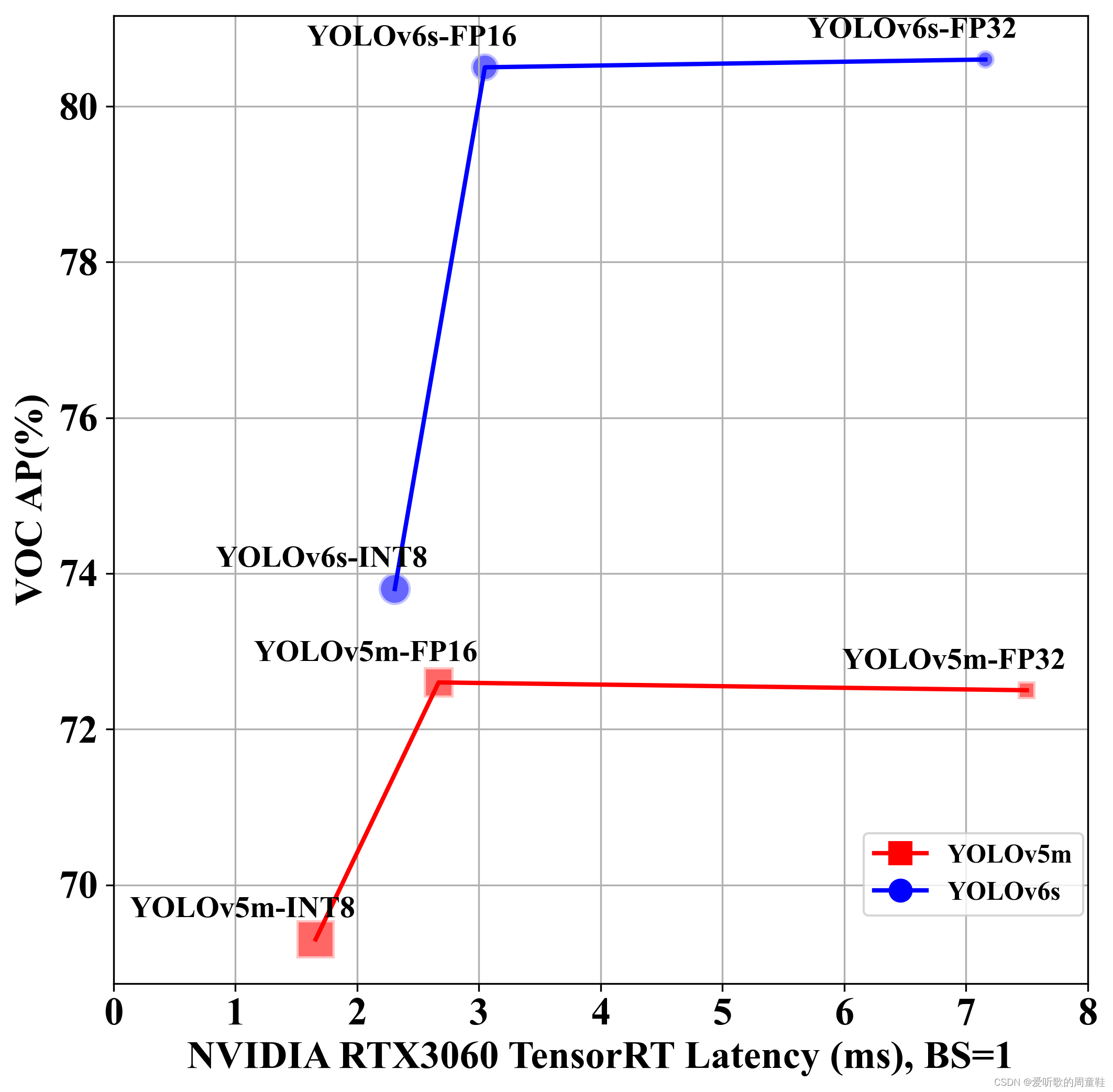
上图中横坐标为不同精度模型在 NVIDIA RTX3060 上一张图片的推理耗时,注意这里 YOLOv5m 包含预处理和后处理,而 YOLOv6s 仅包含推理,纵坐标为不同精度模型在 VOC 数据集上的 mAP50,YOLOv5m 模型以红色方块表示,YOLOv6s 模型以蓝色圆圈表示,图标代表着 FPS 的大小,FPS 越大,对应的图标也越大。
结语
本篇博客简单分享了 tensorRT 模型的性能测试,把具体流程走了一遍,博主训练了 YOLOv5m 和 YOLOv6s 两个模型,分别测试了两个模型对应的 FP32、 FP16、INT8 模型在 NVIDIA RTX3060 上的 mAP 和速度,主要是为了让大家对整体流程有一个基本的把握。博主对于 tensorRT 模型性能测试只做了最基础的演示,如果有更多的需求需要各位看官自己去挖掘啦😄。感谢各位看到最后,创作不易,读后有收获的看官请帮忙👍⭐️
下载链接
- YOLOv5和YOLOv6训练好的VOC权重[pwd:yolo]
- YOLOv6_test源码[pwd:yolo]
- 只包含 src、workspace、CMakeLists.txt 三个文件
- src 文件夹下存放着源码
- workspace 文件夹下存放着速度测试用的图片,以及一些工具测试代码如 mAP_test、xml2yolo 等
- CMakeLists.txt 按照要求修改即可


 4274
4274


 被折叠的 条评论
为什么被折叠?
被折叠的 条评论
为什么被折叠?
 到【灌水乐园】发言


