Image Characteristics Extraction ——Learning notes 1

What is Image Characteristics Extraction?

Image Characteristics Extraction is an important technique for Object Detection. For example, how to recognize the car and how to let the computer understand our brain’s definition of the car with wheels, flat, lights, Windows, etc.? It requires us to extract the characteristics of these objects and translate them into machine language, so that they can be recognized by the computer. Feature extraction is to judge whether the points of the image belong to the features of an image. In this case, I think it can also be called a place we are interested in. So, where in an image are we interested in?

In generally, it can be divided into the following characteristics:
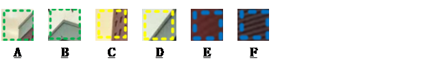
1、 A, B – Corner Point, it is the corner between the two boundaries.
2、C, D – Edge, it is the boundary between two objects.
3、E, F – Area, It’s inside an object.

How to extract the features of the image?

Here, I will introduce three methods of Image Characteristics Extraction. There are Hog feature detection and Harris corner detection.

1、Hog feature detection

Hog, Histogram of Gradient, is using gradient to describe the characteristics of the picture. Its basic principle is to calculate the gradient vector of each point in the specified area of the image and describe this area with gradient histogram. Therefore, it is necessary to know how the gradient is defined. Here are the steps about how it works.

• Image preprocessing

This step is to reduce the noise in the picture. In fact, most images will have noise spots, and these spots will affect the computer’s perception of the image features. Therefore, we need to filter the original image, which can be image morphological processing, gaussian filtering and so on.

• Gradient computation

Now, there is a pixel point (x, y), and it moves Δx in the X-axis, so:

In the same way, we can also get the gradient in the y-direction:

Then, we can get the amplitude and direction of the gradient at this point:

• Cell division

And than we could be divided the image into the same size and non-overlapping regions, which we call it cell. After we’ve computed all the cells, we can divide it into 9 portions depending on the direction of the gradient. And according to the magnitude of the gradient, we can do a weighted statistics for each cell. Therefor, we can get the gradient histogram or vector diagram of the all cell. Now, we can replace the features of a cell or an image with these 9 values.

• Normalization processing

When we have computed the eigenvectors of all cells, we have actually obtained the subsets of the hog characteristic set. And then, we will build blocks by concatenating the features of several cells. And we will normalize the block in order to make the feature vector space has a better robustness to illumination, shadow and edge changes get the hog feature.

The code implementation is as follows:

import cv2
import numpy as np
import math
import matplotlib.pyplot as plt
import seaborn as sns

def cv_show(name, img):     # 图片展示
    cv2.imshow(name, img)
    cv2.waitKey(0)
    cv2.destroyAllWindows()

img = cv2.imread('IMG_20200202_1.jpg', cv2.IMREAD_GRAYSCALE)

sobelx1 = cv2.Sobel(img, cv2.CV_64F, 1, 0, ksize=3)      # 计算x，y方向的梯度幅值
sobelx = cv2.convertScaleAbs(sobelx1)
sobely1 = cv2.Sobel(img, cv2.CV_64F, 0, 1, ksize=3)
sobely = cv2.convertScaleAbs(sobely1)
sobelxy = cv2.addWeighted(sobelx, 0.5, sobely, 0.5, 0)

h, w = img.shape      # 调整图片大小
sobelx = cv2.resize(sobelx, (int(0.3*w), int(0.3*h)))
sobelx1 = cv2.resize(sobelx1, (int(0.3*w), int(0.3*h)))
sobely = cv2.resize(sobely, (int(0.3*w), int(0.3*h)))
sobely1 = cv2.resize(sobely1, (int(0.3*w), int(0.3*h)))
sobelxy = cv2.resize(sobelxy, (int(0.3*w), int(0.3*h)))

cv_show("sobelx", sobelx)
cv_show("sobely", sobely)
cv_show("sobelxy", sobelxy)
str1 = ['x', 'y', 'xy']
names = locals()
for i in range(3):
    filename = 'sobel_' + str1[i] + '.jpg'
    cv2.imwrite(filename, names['sobel%s' % str1[i]])

gradient_angle = cv2.phase(sobelx1, sobely1, angleInDegrees=True)     # 计算梯度方向
h1, w1 = sobelxy.shape
cell_size = 8
bin_size = 9
angle_unit = 360 / bin_size
gradient_magnitude = abs(sobelxy)
cell_gradient_vector = np.zeros((int(h1 / cell_size), int(w1 / cell_size), bin_size))
statistical_result = np.zeros((int(h1 / cell_size), int(w1 / cell_size), bin_size))

def cell_gradient(cell_magnitude, cell_angle):
    # 取cell元素，计算加权梯度直方图
    orientation_centers = [0] * bin_size
    for k in range(cell_magnitude.shape[0]):
        for l in range(cell_magnitude.shape[1]):
            gradient_strength = cell_magnitude[k][l]
            gradient_angle = cell_angle[k][l]
            L_angle = int(gradient_angle / angle_unit) % 9
            R_angle = (L_angle + 1) % bin_size
            mod = gradient_angle % angle_unit
            orientation_centers[L_angle] += (gradient_strength * (1 - (mod / angle_unit)))  # 权重计算
            orientation_centers[R_angle] += (gradient_strength * (mod / angle_unit))
    return orientation_centers
for i in range(cell_gradient_vector.shape[0]):
    # 取cell
    for j in range(cell_gradient_vector.shape[1]):
        cell_magnitude = gradient_magnitude[i * cell_size:(i + 1) * cell_size,
                         j * cell_size:(j + 1) * cell_size]
        cell_angle = gradient_angle[i * cell_size:(i + 1) * cell_size,
                     j * cell_size:(j + 1) * cell_size]
        statistical_result[i][j] = cell_gradient(cell_magnitude, cell_angle)

hog_image = np.zeros([h1, w1])      # hog特征展示
cell_width = cell_size / 2
max_mag = np.array(statistical_result).max()
for x in range(statistical_result.shape[0]):
    for y in range(statistical_result.shape[1]):
        cell_grad = statistical_result[x][y]
        cell_grad /= max_mag
        angle = 0
        angle_gap = angle_unit
        for magnitude in cell_grad:
            angle_radian = math.radians(angle)
            x1 = int(x * cell_size + magnitude * cell_width * math.cos(angle_radian))
            y1 = int(y * cell_size + magnitude * cell_width * math.sin(angle_radian))
            x2 = int(x * cell_size - magnitude * cell_width * math.cos(angle_radian))
            y2 = int(y * cell_size - magnitude * cell_width * math.sin(angle_radian))
            cv2.line(hog_image, (y1, x1), (y2, x2), int(255 * math.sqrt(magnitude)))
            angle += angle_gap

plt.imshow(hog_image, cmap=plt.cm.gray)
plt.xticks([])
plt.yticks([])
plt.show()

Results:

Therefore, we can draw the edge of the object with the hog feature, and use a feature matrix to describe an image.

2、Harris feature detection

Although the Harris feature and the hog feature are two kinds of features, it seems to me that if you already understand the hog feature, the Harris feature will be quite simple.
First of all, the Harris feature is also called corner detection. So let’s go back to the definition of the gradient, and try to find the difference of the gradient for the different feature.

Obviously, we can see that:
1)If it’s an corner point, its gradient will vary dramatically in both directions, such as A and B.
2)If it is a boundary, the gradient of the point at this boundary should vary dramatically in one direction, such as C and D.
3)If it’s a area, then the gradient at all of these area should be flat, like E, F.
Therefore, this problem becomes to build a model describing the rate of gradient change. For this purpose, it establishes a self-similarity function for a pixel, (x, y):

And then we do a Taylor expansion for I(u+Δx, v+Δy), ignore the higher order terms, leaving the first order term only, so:
Finally, we convert it to matrix form, so:

So, this function is converted to a function of an ellipse, and c(x, y; Δx, Δy) becomes the target function. Here, we can do this one operation:

In this case, we can find that the size of c(x, y; Δx, Δy) is only relevant to λ1 and λ2. So, the scientists came up with an R (corner) value corresponding for it:

1)If R > 0 , that means it’s a corner point.
2)If R ≈ 0 , that means it’s a boundary.
3)If R < 0 , that means it’s an area.

Although the derivation of the principle is complicated, opencv-python gives us a function to do this:

cv2.cornerHarris()
'''
img： 数据类型为 float32 的入图像
blockSize： 角点检测中指定区域的大小
ksize： Sobel求导中使用的窗口大小
k： 取值参数为 [0,04,0.06]
'''

For example:

import cv2

img = cv2.imread('IMG_20200202_2.jpg')
gray = cv2.cvtColor(img, cv2.COLOR_BGR2GRAY)
dst = cv2.cornerHarris(gray, 2, 3, 0.04)
img[dst > 0.01*dst.max()] = [0, 0, 255]
cv2.imshow('bookcase', img)
cv2.waitKey(0)
cv2.destroyAllWindows()

Result:

The statement: all materials are used as learning materials only, if the picture involves infringement, please contact me to delete.