数字图像处理课程实验代码

数字图像处理实验

实验要求

1.空域图像增强
（1）直方图均衡化：读入图像，对它做直方图均衡化
（2）点运算
（3）边缘检测：读入图像，用边缘检测算子提取边缘，将原图和其检测出的边缘显示
2.空域图像恢复
（1）去噪：对图像加入高斯和椒盐噪声，用平均值滤波（高斯滤波、中值滤波）、自适应中值滤波进行去噪
（2）去模糊：对图像进行模糊退化，然后去模糊
3.变换域图像增强
（1）FFT： 对图像做傅里叶变换，显示其幅值其相位
（2）WT： 对图像做3尺度的小波变换

用matlab实现

代码部分

%% 直方图均衡化
A=imread('D:\数字图像处理\IMG.jpg');%此处为处理图片的保存位置
B=rgb2gray(A);   %原图（灰度图）
figure,subplot(2,2,1),imshow(B);
subplot(2,2,2),imhist(B);  
title('原图及其直方图'); 
C=histeq(B);
subplot(2,2,3),imshow(C);
subplot(2,2,4),imhist(C);
title('均衡化及其直方图');
%% 对比度拉伸（点运算）
s=imadjust(B,[0.2 0.5],[0 1]);%将0.2-0.5之间的灰度扩展到整个0-1范围，这种处理对于强调感兴趣灰度区非常有用
% set(0,'defaultFigurePosition',[100,100,1000,500]);
% set(0,'defaultFigureColor',[1 1 1]);
figure,
subplot(121),imshow(B),title('原图'); 
subplot(122),imshow(s),title('点运算');


%% 边缘检测
% BW=edge(C,'roberts',0.1);%roberts梯度
% figure,imshow(BW);
H=[0 -1 0;-1 4 -1;0 -1 0];%LPLS算子
J=imfilter(B,H);
figure,subplot(2,2,1),imshow(B);title('原图'); 
subplot(2,2,2),imhist(B);title('原图直方图'); 
subplot(2,2,3),imshow(J);title('边缘检测'); 
subplot(2,2,4),imhist(J);title('边缘检测直方图'); 
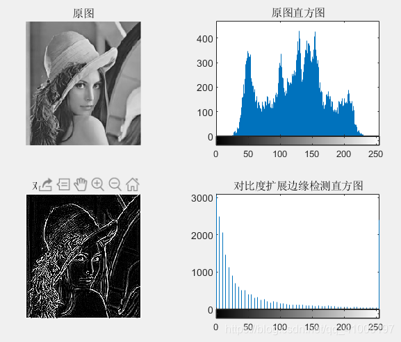
K=imadjust(J,[0.0 0.2],[]);
figure,subplot(2,2,1),imshow(B);title('原图'); 
subplot(2,2,2),imhist(B);title('原图直方图'); 
subplot(2,2,3),imshow(K);title('对比度扩展边缘检测'); 
subplot(2,2,4),imhist(K); title('对比度扩展边缘检测直方图'); 

%% 去噪
f=imnoise(B,'salt & pepper',0.04); %f为加噪后图像

% h0=1/9.*[1 1 1 1 1 1 1 1 1];
% h1=[0.1 0.1 0.1;0.1 0.2 0.1;0.1 0.1 0.1];
h2=1/16.*[1 2 1;2 4 2;1 2 1];%高斯滤波
% h3=1/8.*[1 1 1;1 0 1;1 1 1];
% g0=filter2(h0,f);
% g1=filter2(h1,f);
g2=filter2(h2,f);
% g3=filter2(h3,f);
% figure,imshow(g0,[]);
% figure,imshow(g1,[]);
% figure,imshow(g2,[]);
% % figure,imshow(g3,[]);
% title('高斯滤波');

k=medfilt2(f);%二维中值滤波
% figure;imshow(k);
% title('二维中值滤波');

p=adpmedian(f,11);
% figure;imshow(p);
% title('自适应中值滤波');


figure,subplot(2,2,1),imshow(f),title('加入椒盐噪声');
subplot(2,2,2),imshow(g2,[]),title('高斯滤波');
subplot(2,2,3),imshow(k),title('二维中值滤波');
subplot(2,2,4),imshow(p),title('自适应中值滤波'); 
%% 去模糊
psf=fspecial('gaussian',7,0.8);
blurred=imfilter(B,psf);
wnrl=deconvwnr(blurred,psf);
figure,
subplot(131),imshow(B),title('原图');
subplot(132),imshow(blurred),title('高斯模糊');
subplot(133),imshow(wnrl),title('维纳滤波');
%% fft
f=fft2(B); %傅里叶变换
f=fftshift(f); %使图像对称
r=real(f); %图像频域实部
i=imag(f); %图像频域虚部
margin=log(abs(f)); %图像幅度谱，加log便于显示
phase=log(angle(f)*180/pi); %图像相位谱
l=log(f); 
figure,
subplot(2,2,1),imshow(B),title('原图');
subplot(2,2,2),imshow(l,[]),title('图像频谱');
subplot(2,2,3),imshow(margin,[]),title('图像幅度谱');
subplot(2,2,4),imshow(phase,[]),title('图像相位谱');
%% 小波
[X,map]=gray2ind(B,128);
[c,s]=wavedec2(X,3,'haar');
ca3=appcoef2(c,s,'haar',3);
ca2=appcoef2(c,s,'haar',2);
ca1=appcoef2(c,s,'haar',1);
figure,title('低频系数'),
subplot(3,4,1),imshow(ca1,[]);
subplot(3,4,5),imshow(ca2,[]);title('第二尺度低频系数'),
subplot(3,4,9),imshow(ca3,[]);


ch3=detcoef2('h',c,s,3);
ch2=detcoef2('h',c,s,2);
ch1=detcoef2('h',c,s,1);

cv3=detcoef2('v',c,s,3);
cv2=detcoef2('v',c,s,2);
cv1=detcoef2('v',c,s,1);

cd3=detcoef2('d',c,s,3);
cd2=detcoef2('d',c,s,2);
cd1=detcoef2('d',c,s,1);

subplot(3,4,2),imshow(ch1,[]);title('第一尺度水平高频系数'),
subplot(3,4,6),imshow(ch2,[]);title('第二尺度水平高频系数'),
subplot(3,4,10),imshow(ch3,[]);title('第三尺度水平高频系数'),

subplot(3,4,3),imshow(cv1,[]);title('第一尺度垂直高频系数'),
subplot(3,4,7),imshow(cv2,[]);title('第二尺度垂直高频系数'),
subplot(3,4,11),imshow(cv3,[]);title('第三尺度垂直高频系数'),

subplot(3,4,4),imshow(cd1,[]);title('第一尺度对角高频系数')
subplot(3,4,8),imshow(cd2,[]);title('第二尺度对角高频系数'),
subplot(3,4,12),imshow(cd3,[]);title('第三尺度对角高频系数')

function f =adpmedian(g,Smax)
if(Smax<=1)||(Smax/2==round(Smax/2))||(Smax~=round(Smax))
    error('SMAX must be an odd integer>1.')
end
f =g;
f(:)=0;
alreadyProcessed=false(size(g));
for k=3:2:Smax
    zmin=ordfilt2(g,1,ones(k,k),'symmetric');
    zmax=ordfilt2(g,k*k,ones(k,k),'symmetric');
    zmed=medfilt2(g,[k k],'symmetric');
    
    processUsingLevelB =(zmed>zmin) & (zmax>zmed) & ...
        ~ alreadyProcessed;
    zB=(g>zmin)&(zmax>g);
    outputZxy=processUsingLevelB & zB;
    outputZmed=processUsingLevelB & ~zB;
    f(outputZxy)=g(outputZxy);
    f(outputZmed)=zmed(outputZmed);
    
    alreadyProcessed=alreadyProcessed|processUsingLevelB;
    if all(alreadyProcessed(:))
        break;
    end
end
f(~alreadyProcessed)=zmed(~alreadyProcessed);

仿真时使用的图片，可以使用其他图片，不过要注意图片的大小，否则可能报错

运行结果

1.原图及其直方图

2.均衡化处理后图及其直方图

3.点运算处理

4.边缘检测及其直方图

5.对比度扩展边缘检测直方图

6.给图像加入椒盐噪声并分别进行高斯滤波、二维中值滤波、自适应中值滤波处理

7.加入高斯模糊并进行维纳滤波处理

8.对图像做傅里叶变换，显示其幅值其相位

9.对图像做3尺度的小波变换，提取高、低频系数